Download
1 / 56
560 likes | 762 Vues
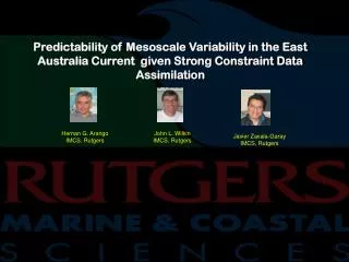
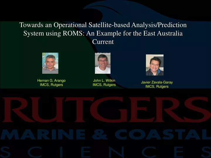
Towards an Operational Satellite-based Analysis/Prediction System using ROMS: An Example for the East Australia Current. Hernan G. Arango IMCS, Rutgers. John L. Wilkin IMCS, Rutgers. Javier Zavala-Garay IMCS, Rutgers. Outline. EAC application Brief summary of IS4DVAR

E N D
Towards an Operational Satellite-based Analysis/Prediction System using ROMS: An Example for the East Australia Current Hernan G. Arango IMCS, Rutgers John L. Wilkin IMCS, Rutgers Javier Zavala-Garay IMCS, Rutgers
Outline • EAC application • Brief summary of IS4DVAR • Updated version on EAC-IS4DVAR analysis/prediction system • Background error covariance modeling • Some preliminary results • Future work
-24 -28 -32 -36 -40 -44 -48 165 155 150 160 145 East Australia Current Application Configuration
IS4DVAR • Given a first guess (a forward trajectory)
IS4DVAR • Given a first guess (a forward trajectory)… • And given the available data…
IS4DVAR • Given a first guess (a forward trajectory)… • And given the available data… • What are the changes (or increment) to the IC so that the forward model fits the observations?
The best fit becomes the reanalysis assimilation window
The final state becomes the IC for the forecast window assimilation window forecast
The final state becomes the IC for the forecast window assimilation window forecast verification
4DVar Observations XBTs We have moved from SSH 7-Day Averaged AVISO To SSH 4-day avg. from CSIRO (compatible with SXBT=SCTD) SST Daily CSIRO Days since January 1st 2001, 00:00:00
EAC Incremental 4DVar: Surface Versus Sub-surface Observations
EAC Incremental 4DVar: Surface Versus Sub-surface Observations First Guess SSH/SST
EAC Incremental 4DVar: Surface Versus Sub-surface Observations Observations SSH/SST First Guess SSH/SST
EAC Incremental 4DVar: Surface Versus Sub-surface Observations Observations ROMS IS4DVAR: SSH/SST SSH/SST SSH/SST First Guess ROMS IS4DVAR: XBT Only SSH/SST SSH/SST
Comparison between ROMS fit and observed temperature from all XBTs. Note: actual XBT-data was not assimilated, it is used here to evaluate the quality of the reanalysis. SSH+SST
Comparison between ROMS fit and observed temperature from all XBTs. Note: actual XBT-data was not assimilated, it is used here to evaluate the quality of the reanalysis. SSH+SST Assimilation of SST
Comparison between ROMS fit and observed temperature from all XBTs. Note: actual XBT-data was not assimilated, it is used here to evaluate the quality of the reanalysis. SSH+SST Assimilation of SST Erroneousprojection of SSH information
Comparison between ROMS fit and observed temperature from all XBTs. Note: actual XBT-data was not assimilated, it is used here to evaluate the quality of the reanalysis. SSH+SST SSH+SST+SynXBT
Comparison between ROMS prediction and observed temperature from all XBTs.
Comparison between ROMS prediction and observed temperature from all XBTs.
Comparison between ROMS prediction and observed temperature from all XBTs.
Comparison between ROMS prediction and observed temperature from all XBTs.
Comparison between ROMS prediction and observed temperature from all XBTs.
some remarks • Good ocean state predictions for up to 2 weeks in advance • Need to correctly project the altimeter data • Proxies for subsurface information can be obtained based on surface information, but need lots of subsurface data to construct a robust empirical relationship • The fact that an empirical (linear) relationship exist suggest that there could be a simple dynamical relationships linking the surface with the subsurface variability • The idea is actually not new (Weaver et al 2006: “multivariate balance operator”)
What we have learned • Need a good unbiased background or first guess • From a “good” model forced by unbiased boundary and surface forcing • From assimilation of climatological seasonal cycle of T and S (e.g. Levitus, CARS). • Adequate modeling the background error covariance B is a crucial. • So far, to model B we need to specify • Spatial decorrelation scales • Standard deviations of the increments.
How can the information content of one variable be transferred to other variables? • Two possibilities: 1) Using the adjoint model 2) Modeling of the background covariance matrix
Balance operator for mesoscale variability • Forward problem (scalar SSH given a vector dT) • Given dT (e.g., XBT) • Find dS • Find density anomalies • Find SHH. • Inverse problem (given scalar SSH guess the vectors dT and dS).