Download
1 / 27
270 likes | 438 Vues
Prediction of Ocean Circulation in the Gulf of Mexico and Caribbean Sea An application of the ROMS/TOMS Data Assimilation Models. Hernan G. Arango (IMCS, Rutgers University) Emanuele Di Lorenzo (Georgia Institute of Technology) Arthur J. Miller, Bruce D. Cornuelle

E N D
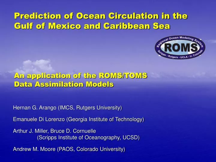
Prediction of Ocean Circulation in the Gulf of Mexico and Caribbean SeaAn application of the ROMS/TOMS Data Assimilation Models Hernan G. Arango (IMCS, Rutgers University) Emanuele Di Lorenzo (Georgia Institute of Technology) Arthur J. Miller, Bruce D. Cornuelle (Scripps Institute of Oceanography, UCSD) Andrew M. Moore (PAOS, Colorado University)
Ocean Observations Gulf of Mexico and Caribbean Seas plus satellite data (SSH, SST) and radar
Ocean Modeling Framework ROMS/TOMS
Ocean Modeling of North Atlantic Gulf of Mexico Ocean Model Grid
Ocean Modeling Applications in Gulf of Mexico and Caribbean Seas • Develop a real-time data assimilation and prediction system for the Gulf of Mexico and Caribbean Seas based on a continuous upper ocean monitoring system • Demonstrate the utility of variational data assimilation in a real-time, sea-going environment • Demonstrate the value of collecting routine ocean observations from specially equipped ocean vessels (Explorer of the Seas) • Develop much needed experience in both the assimilation of disparate ocean data and ocean prediction in regional ocean models. • Add platform oceanic measurements (a possibility)
Ensemble Prediction For an appropriate forecast skill measure, s
Ocean Adjoint Modeling Applications Example from the Caribbean model run, of sensitivity of the transport through the Yucatan Strait given a particular realization of the circulation. In this case the maximum transport at time tN, indicated by the strong gradients in sea surface height (SSH), is sensitive to a pattern of Kelvin waves at previous time t0. These types of sensitivity, computed using the non-linear and Adjoint models of ROMS, will be applied for the Florida Strait to explore how different topographic shapes affect the transport during different circulation regimes.
4D Variational Data Assimilation Platforms (4DVAR) • Strong Constraint (S4DVAR) drivers: • Conventional S4DVAR: outer loop, NLM, ADM • Incremental S4DVAR: inner and outer loops, NLM, TLM, ADM (Courtier et al., 1994) • Efficient Incremental S4DVAR (Weaver et al., 2003) • Weak Constraint (W4DVAR) - IOM • Indirect Representer Method: inner and outer loops, NLM, TLM, RPM, ADM (Egbert et al., 1994; Bennett et al, 1997)
Strong Constraint 4DVAR from IOM (Di Lorenzo et al., 2005)
T Assimilated data: TS 0-500m Free surface Currents 0-150m S V U True Synthetic Data Strong Constraint SST SST 1st Guess Weak Constraint SST SST Strong and Weak Constraint 4DVAR (Southern California Bight) Normalized Misfit Datum 0-500 m data CalCOFI Sampling grid Annual Climatology
Adjoint Sensitivity • Given the model state vector: • Consider a Yucatan Strait transport index, , defined in terms of space and/or time integrals of : • Small changes in will lead to changes in where: • We will define sensitivity as etc. + …
Publications Arango, H.G., Moore, A.M., E. Di Lorenzo, B.D. Cornuelle, A.J. Miller and D. Neilson, 2003: The ROMS Tangent Linear and Adjoint Models: A comprehensive ocean prediction and analysis system, Rutgers Tech. Report. http://marine.rutgers.edu/po/Papers/roms_adjoint.pdf Di Lorenzo, E., A.M. Moore, H.G. Arango, B. Chua, B.D. Cornuelle, A.J. Miller and A. Bennett, 2005: The Inverse Regional Ocean Modeling System: Development and Application to Data Assimilation of Coastal Mesoscale Eddies, Ocean Modelling, In preparation. Moore, A.M., H.G Arango, E. Di Lorenzo, B.D. Cornuelle, A.J. Miller and D. Neilson, 2004: A comprehensive ocean prediction and analysis system based on the tangent linear and adjoint of a regional ocean model, Ocean Modelling, 7, 227-258. http://marine.rutgers.edu/po/Papers/Moore_2004_om.pdf Moore, A.M., E. Di Lorenzo, H.G. Arango, C.V. Lewis, T.M. Powell, A.J. Miller and B.D. Cornuelle, 2005: An Adjoint Sensitivity Analysis of the Southern California Current Circulation and Ecosystem, J. Phys.Oceanogr., In preparation. Wilkin, J.L., H.G. Arango, D.B. Haidvogel, C.S. Lichtenwalner, S.M.Durski, and K.S. Hedstrom, 2005: A Regional Modeling System for the Long-term Ecosystem Observatory, J. Geophys. Res., 110, C06S91, doi:10.1029/2003JCC002218. http://marine.rutgers.edu/po/Papers/Wilkin_2005_jgr.pdf Warner, J.C., C.R. Sherwood, H.G. Arango, and R.P. Signell, 2005: Performance of Four Turbulence Closure Methods Implemented Using a Generic Length Scale Method, Ocean Modelling, 8, 81-113. http://marine.rutgers.edu/po/Papers/Warner_2004_om.pdf
Let’s represent NLM ROMS as: • The TLM ROMS is derived by considering a small perturbation sto S. A first-order Taylor expansion yields: A is real, non-symmetricPropagator Matrix • The ADM ROMS is derived by taking the inner-product with an arbitrary vector , where the inner-product defines an appropriate norm (L2-norm): Overview
Eigenmodes of and Tangent Linear and Adjoint Based GST Drivers • Singular vectors: • Forcing Singular vectors: • Stochastic optimals: • Pseudospectra:
Two Interpretations • Dynamics/sensitivity/stability of flow to naturally occurring perturbations • Dynamics/sensitivity/stability due to error or uncertainties in the forecast system • Practical applications: • Ensemble prediction • Adaptive observations • Array design ...
SST and Surface currents Free-Surface GSA on the Southern California Bight (SCB)
TLM eigenvectors (A): normal modes • ADM eigenvectors (AT): optimal excitations Real Part Imag Part SCB coastally trapped waves Eigenmodes
Optimal Perturbations diffluence • A measurement of the fastest growing of all possible perturbations over a given time interval confluence SCB maximum growth of perturbation energy over 5 days
Stochastic Optimals Provide information about the influence of stochastic variations (biases) in ocean forcing SCB patterns of stochastic forcing that maximizes the perturbation energy variance for 5 days
Singular Vectors Open Boundary Sensitivity: errorsgrowth quickly and appear to propagate through the model domain as coastally trapped waves.
Ensemble Prediction • Optimal perturbations / singular vectors and stochastic optimal can also be used to generate ensemble forecasts. • Perturbing the system along the most unstable directions of the state space yields information about the first and second moments of the probability density function (PDF): • ensemble mean • ensemble spread • Adjoint based perturbations excite the full spectrum
where model, background, observations, inverse background error covariance, inverse observations error covariance • Model solution depends on initial conditions ( ), boundary conditions, and model parameters • Minimize J to produce a best fit between model and observations by adjusting initial conditions, and/or boundary conditions, and/or model parameters. Data Assimilation Overview • Cost Function:
We require the minimum of at which: , , , yielding • AT is the transpose of A, often called the adjoint operator. It can be shown that: The adjoint equation solution provides gradient information Minimization • Perfect model constrained minimization (Lagrange function):
RP: 4D Variational Data Assimilation Platforms (4DVAR) • Strong Constraint (S4DVAR) drivers: • Conventional S4DVAR: outer loop, NLM, ADM • Incremental S4DVAR: inner and outer loops, NLM, TLM, ADM (Courtier et al., 1994) • Efficient Incremental S4DVAR (Weaver et al., 2003) • Weak Constraint (W4DVAR) - IOM • Indirect Representer Method: inner and outer loops, NLM, TLM, RPM, ADM (Egbert et al., 1994; Bennett et al, 1997)
Forward and Adjoint MPI Communications Forward Adjoint