Download
1 / 24
240 likes | 333 Vues
Soil Moisture Algorithm Results Oklahoma H Polarization. DMSP Special Sensor Microwave/Imager (SSM/I). Shown here are 1.4 GHz results obtained using an aircraft sensor and 19 GHz satellite data The difference between the sensitivity of the two instruments is quite apparent

E N D
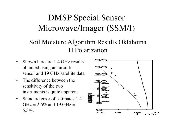
Soil Moisture Algorithm Results OklahomaH Polarization DMSP Special Sensor Microwave/Imager (SSM/I) • Shown here are 1.4 GHz results obtained using an aircraft sensor and 19 GHz satellite data • The difference between the sensitivity of the two instruments is quite apparent • Standard error of estimates:1.4 GHz = 2.6% and 19 GHz = 5.3%.
Heavy Vegetation Light Vegetation Good dynamic range over lightly vegetated surfaces AMSR-E 10.4 GHz AMSR-E 10.4 GHz PrincetonUniversity Soil moisture Soil moisture Sensitivity of microwave brightness temperature to soil moisture (SGP’97) ESTAR 1.4 GHz SSM/I 19 GHz Soil moisture Soil moisture Microwave emissions and soil moisture
240 250 260 [oK] TOA brightness temperature TOA brightness temperature PrincetonUniversity AMSR brightness temperature (60 km) AMSR estimated soil moisture (25 km) AMSR-E OSSE for soil moisture Soil Moisture (1 km)
PrincetonUniversity OSSE for AMSR-E Soil Moisture Retrievals
July 4-6 Aqua AMSR Three Day Composite Brightness Temperature
July 4-6 Aqua AMSR Three Day Composite Brightness Temperature
LAND COVER CLASSIFICATION AND NDVI ANALYSIS FOR THE SGP 1999 EXPERIMENT AREA INTRODUCTION One of the goals of the Southern Great Plains 1999 (SGP99) Hydrology Experiment is to obtain information of soil moisture pattern on the regional scale. The soil moisture algorithm based on remote sensing measurements requires land cover information as one of the inputs into the model. Vegetation cover strongly affects the microwave emission from the soil and it is important in soil moisture investigation and analysis LAND COVER CLASSIFICATION AND NDVI
METHOD A land cover study was conducted between July 8 – July 21 1999. For this period, and prior to it, Landsat TM scenes were collected. A ground truth survey was designed based on aerial photographs, which indicated 16 main land cover categories. During the experiment there was some harvesting of wheat, alfalfa and corn. Land cover categories were selected to follow the changes in vegetation cover by distinguishing such classes as bare soil, bare soil with wheat stubble and harvested fields with growing weeds (bare soil with green vegetation). Also, special attention was paid to different types of pasture. Two types of pasture were distinguished – grass areas that are grazed and used as regular pastures and grass areas left idle. The list of 15 land cover categories reflects all the main types of vegetation of the experimental period. Land cover classification was performed based on those images that had the least cloud coverage. From the available Landsat 5 and Landsat 7 TM images, 4 scenes were used – March 9, May 12, July 15 and July 23 1999. Unfortunately, no useful Landsat images for the months of April or June were available
RESULTS The classification results were analyzed using confusion and separability matrices. Battacharrya Distance was used as a separability measure between the categories. Most classes had good separability (above 1.9 on a scale from 0.0 to 2.0). The Normalized Difference Vegetation Index was calculated in order to follow the changes in the biomass during the experimental period. Special attention was paid to those test sites within which sampling of soil moisture was done during the time of experiment. For these locations, analysis of NDVI and vegetation water content will be performed in order assess the optical depth of vegetation layer which have significant influence on microwave emission for the soil.
Alfalfa Bare soil Bare soil with wheat stubble Bare soil with green vegetation Corn Legume Outcrops Pasture grazed Pasture ungrazed Quarries and sand bars Shrubs Trees Urban Water Wheat stubble • LANDSAT TM IMAGES • March 09 1999 • May 12 1999 • July 15 1999 • July 23 1999 • Maximum Likelihood Classification • bands 3,4,5,and 7 for each date • PCIWorks software V.6.3.0 • GROUND SURVEY • July 07-July 20 1999 • based on air-photographs • 1320 individual training sites • originally 44 categories • regrouped to 15 basic land cover classes El Reno test site area with training sites from the ground truth survey
0 Unclassified 1 Alfalfa 2 Bare soil 3 Bare soil with wheat stubb. 4 Bare soil with green veg. 5 Corn 6 Legume 7 Outcrops 8 Pasture grazed 9 Pasture ungrazed 10 Quarries and sand bars 11 Shrubs 12 Trees 13 Urban 14 Water 15 Wheat stubble Landcover categories ER20 ER18 ER19 ER01 ER17 ER05 Results of land cover classification for El Reno test site area
NDVI temporal analysis allows for detecting seasonal changes in biomass and helps in assigning the vegetation parameters derived from land cover categories, that are needed for the soil moisture algorithm calculation
1 0 NDVI of July 15 for El Reno test site area Land cover and NDVI data can be found on the web site of GSFC Earth Sciences Distributed Active Archive Center: http://daac.gsfc.nasa.gov/CAMPAIGN_DOCS/ SGP99/veg_cov.html NDVI image calculated from Landsat 5 TM July 15 1999
USING GIS IN SOIL MOISTURE RETRIEVAL BASED ON PASSIVE MICROWAVE REMOTE SENSING
INTRODUCTION Soil moisture is very important in hydrology, agriculture and land management but is difficult to measure using conventional methods. Remote sensing, in particular passive microwave, has a great potential for providing areal estimates of soil moisture. An example of how passive microwave soil moisture mapping could be implemented with aircraft based sensors is described here. During the Southern Great Plains’97 Hydrology Experiment, a passive microwave imaging instrument operating at =21 cm was used for measuring soil brightness temperature. The equipment - Electronically Scanned Thinned Radiometer (ESTAR) - was deployed on a NASA P-3 aircraft. The images of brightness temperature can be converted to volumetric soil moisture maps using additional environmental information and a Geographical Information Systems (GIS). The experimental region, marked as a black rectangular on the picture, is more then 10,000-sq. km in size. In order to illustrate the changes in soil moisture pattern on the local scale, the area of the Little Washita watershed was chosen for this presentation.
Altitude ~ 7.6 km Brightness temperature image on June 30th Irregular grid of brightness temperature measurements Result - uniform data layers with brightness temperature - for the each day of the experiment DATA INPUT Brightness Temperature Data Data re-gridded to 200-m resolution NASA P-3 aircraft with passive microwave radiometer operating at 1.415 GHz (L band) Data from point measurements - Oklahoma Mesonet stations DATA INPUT Soil Temperature Data Soil temperature on June 30th Data re-gridded to 200-m resolution Result - uniform data layers with soil temperature - for the each day of the experiment >24.9°C <23,7° C Land Cover Categories from Landsat TM Classification Attribute data assignment to land cover categories in 30 x 30 m grid DATA INPUT Thematic Mapper Images Bulk density NDVI image Vegetation parameter Data of each data layer averaged for 6 x 6 pixel blocks DATA INPUT Ground Measurements of Vegetation Water Content (VWC) Relationship between vegetation water content and NDVI for grass areas VWC = f(NDVI) Surface roughness 6 output data layers - constant values for the whole experimental period Vegetation water content Resampling original grid to 200m Soil texture classes of the top layer (0-5 cm) Sand Sandy Loam Loam Silt Loam Silty Clay Loam Clay Loam Silty Clay Clay Loamy Sand DATA INPUT Soil Texture Categories Attribute data assignment to texture categories in 200 m grid % clay content % sand content GEOGRAPHICAL DATA BASE
June 29 SOIL MOISTURE ALGORITHM CALCULATIONS USING GIS The soil moisture algorithm requires the remotely sensed input data layer (the soil brightness temperature), and also the physical temperature of the soil and additional environmental data layers, as shown on the adjacent flowchart. The Geographical Information System facilitated the processing and computation. All data layers were combined together in order to generate the final product – soil moisture maps over the investigated area. June 30 July 01 SOIL MOISTURE ALGORITHM CALCULATIONS July 02 July 03 Volumetric Soil Moisture >50% <5%
RESULTS Images presented here for the Little Washita watershed cover an area of 848.2 sq. km and show the spatial variation of soil moisture on 5 consecutive days. Distinct and consistent spatial patterns are observed in the image sequence. This information would be difficult to obtain using conventional methods. Comparison of soil moisture maps with soil texture classes distribution reveals a close relation between the soil moisture pattern and soils texture. Sandy soils (generally in the central part of the images) are drier at the beginning of the drying down cycle and loose soil moisture faster compared to the adjacent silt loam areas. As the drying period proceeds, all soil types become drier, yet the pattern of soil moisture following soil texture classes can still be easily detected. Land use patterns follow the soil moisture distribution. Comparing the land cover image with soil texture map we can observe that winter wheat occurs on soils that can hold enough water for plant growth. Otherwise, land cover is generally grass and shrubs. Passive microwave remote sensing measurements offer an efficient way of obtaining information on soil moisture distribution over space and time. An aircraft based system can provide information on the soil moisture distribution at local and regional scales. In the near future spaceborne instruments will have the ability to measure soil moisture dynamics on the global scale.
The potential for a space-borne Global Water Cycle observation system PrincetonUniversity Radiation (CERES) Snow (AMSR) Vegetation (MODIS) Soil moisture (AMSR) Clouds Soil moisture Precipitation (liquid) Current missions have a capacity to monitor water cycle. Missing global observations: River/lake monitoring,Precipitation, Soil Moisture, Snow
Global Precipitation Mission (GPM) Reference Concept PrincetonUniversity
GPM Systematic Measurement Coverage(Core + 6 constellation members) PrincetonUniversity GPM Core + DMSP(F18) + DMSP(F19) + GCOM-B1 + NASA-GPM I + Euro-GPM I + Euro-GPM II 3-hour sensor ground trace
Soil Moisture and Freeze-Thaw States: HYDROS: Hydrosphere StateMission PrincetonUniversity MEASUREMENTS: • L-band active and passive • Soil moisture: 10-40km • (2-3 day revisit) • Freeze-thaw : 3 km • (1-2 day revisit) Hydrosphere Mission
Observing rivers and water bodies from space: Hydrologic Altimetry Mission PrincetonUniversity