Download
1 / 44
440 likes | 606 Vues
Packet Switching. Not All Networks Are Directly Connected. Outline. Switching and Forwarding Bridges and LAN Switches Cell Switching (ATM) Implementation and Performance. T3. T3. Switch. T3. T3. STS-1. STS-1. Input. Output. ports. ports. Scalable Networks. Switch

E N D
Packet Switching Not All Networks Are Directly Connected
Outline • Switching and Forwarding • Bridges and LAN Switches • Cell Switching (ATM) • Implementation and Performance
T3 T3 Switch T3 T3 STS-1 STS-1 Input Output ports ports Scalable Networks • Switch • forwards packets from input port to output port • port selected based on address in packet header • Advantages • cover large geographic area (tolerate latency) • support large numbers of hosts (scalable bandwidth)
0 Switch 1 3 1 2 Switch 2 2 3 1 5 11 0 Host A 7 0 Switch 3 1 3 4 Host B 2 Virtual Circuit Switching • Explicit connection setup (and tear-down) phase • Subsequence packets follow same circuit • Sometimes called connection-oriented model • Analogy: phone call • Each switch maintains a VC table
Host D Host E 0 Switch 1 Host F 3 1 Switch 2 2 Host C 2 3 1 0 Host A 0 Switch 3 Host B Host G 1 3 2 Host H Datagram Switching • No connection setup phase • Each packet forwarded independently • Sometimes called connectionless model • Analogy: postal system • Each switch maintains a forwarding (routing) table
Circuit Table (switch 1, port 2) Forwarding Table (switch 1) Example Tables
Virtual Circuit Model • Typically wait full RTT for connection setup before sending first data packet. • While the connection request contains the full address for destination, each data packet contains only a small identifier, making the per-packet header overhead small. • If a switch or a link in a connection fails, the connection is broken and a new one needs to be established. • Connection setup provides an opportunity to reserve resources.
Datagram Model • There is no round trip delay waiting for connection setup; a host can send data as soon as it is ready. • Source host has no way of knowing if the network is capable of delivering a packet or if the destination host is even up. • Since packets are treated independently, it is possible to route around link and node failures. • Since every packet must carry the full address of the destination, the overhead per packet is higher than for the connection-oriented model.
Three ways to handle headers • Rotation • Stripping • pointer Header entering D C B A D C B A Ptr D C B A switch Header leaving A D C B D C B Ptr D C B A switch
Outline • Switching and Forwarding • Bridges and LAN Switches • Cell Switching (ATM) • Implementation and Performance
A B C Port 1 Bridge Port 2 Z X Y Bridges and Extended LANs • LANs have physical limitations (e.g., 2500m) • Connect two or more LANs with a bridge • accept and forward strategy • level 2 connection (does not add packet header) • Ethernet Switch = Bridge on Steroids
A B C Port 1 Bridge Port 2 Z X Y Learning Bridges • Do not forward when unnecessary • Maintain forwarding table A 1 B 1 C 1 X 2 Y 2 Z 2 • Learn table entries based on source address • Table is an optimization; need not be complete • Always forward broadcast frames Host Port
A B B3 C B5 D B7 K B2 E F B1 G H B6 B4 I J Spanning Tree Algorithm • Problem: loops exist! • Bridges run a distributed spanning tree algorithm • select which bridges actively forward • developed by Radia Perlman • now IEEE 802.1 specification
Algorithm Overview • Each bridge has unique id (e.g., B1, B2, B3) • Select bridge with smallest id as root • Select bridge on each LAN closest to root as designated bridge (use id to break ties) • Each bridge forwards frames over each LAN for which it is the designated bridge A B B3 C B5 D B7 K B2 E F B1 G H B6 B4 I J
Algorithm Details • Bridges exchange configuration messages • id for bridge sending the message • id for what the sending bridge believes to be root bridge • distance (hops) from sending bridge to root bridge • Each bridge records current best configuration message for each port • Initially, each bridge believes it is the root
Algorithm Detail (cont) • When learn not root, stop generating config messages • in steady state, only root generates configuration messages • When learn not designated bridge, stop forwarding config messages • in steady state, only designated bridges forward config messages • Root continues to periodically send config messages • If any bridge does not receive config message after a period of time, it starts generating config messages claiming to be the root
The limitation of the algorithm Spanning tree algorithm can configure the tree whenever a bridge fails, it can not forward frames over alternative paths for routing around a congested bridge.
Broadcast and Multicast • Forward all broadcast/multicast frames • current practice • Learn when no group members downstream • Accomplished by having each member of group G send a frame to bridge multicast address with G in source field
Limitations of Bridges • Do not scale • spanning tree algorithm does not scale • broadcast does not scale • Do not accommodate heterogeneity • Caution: beware of transparency • It is never safe to design a network software under the assumption that it will run over a single Ethernet segment. Bridges might be used.
W X VLAN 100 VLAN 100 B1 B2 VLAN 200 VLAN 200 Y Z Virtual LAN • VLANs allow a single extended LAN to be partitioned into several seemingly separate LANs. • Packets can only travel between two segments with the same VLAN ID. • VLAN allow us to change the logical topology without moving any wires or changing any addresses.
Outline • Switching and Forwarding • Bridges and LAN Switches • Cell Switching (ATM) • Implementation and Performance
Cell Switching (ATM) • Connection-oriented packet-switched network • Used in both WAN and LAN settings • Signaling (connection setup) Protocol: Q.2931 • Specified by ATM forum • Packets are called cells • 5-byte header + 48-byte payload • Commonly transmitted over SONET • other physical layers possible
Variable vs Fixed-Length Packets • No Optimal Length • if small: high header-to-data overhead • if large: low utilization for small messages • Fixed-Length Easier to Switch in Hardware • simpler • enables parallelism
Big vs Small Packets • Small Improves Queue behavior • finer-grained preemption point for scheduling link • maximum packet = 4KB • link speed = 100Mbps • transmission time = 4096 x 8/100 = 327.68us • high priority packet may sit in the queue 327.68us • in contrast, 53 x 8/100 = 4.24us for ATM • near cut-through behavior • two 4KB packets arrive at same time • link idle for 327.68us while both arrive • at end of 327.68us, still have 8KB to transmit • in contrast, can transmit first cell after 4.24us • at end of 327.68us, just over 4KB left in queue
Big vs Small (cont) • Small Improves Latency (for voice) • voice digitally encoded at 64KBps (8-bit samples at 8KHz) • need full cell’s worth of samples before sending cell • example: 1000-byte cells implies 125ms per cell (too long) • smaller latency implies no need for echo cancellers • ATM Compromise: 48 bytes = (32+64)/2
4 16 3 1 8 8 384 (48 bytes) GFC VPI VCI Type CLP HEC (CRC-8) Payload Cell Format • User-Network Interface (UNI) • host-to-switch format • GFC: Generic Flow Control (still being defined) • VCI: Virtual Circuit Identifier • VPI: Virtual Path Identifier • Type: management, congestion control, AAL5 (later) • CLPL Cell Loss Priority • HEC: Header Error Check (CRC-8) • Network-Network Interface (NNI) • switch-to-switch format • GFC becomes part of VPI field
Segmentation and Reassembly • ATM Adaptation Layer (AAL) • AAL 1 and 2 designed for applications that need guaranteed rate (e.g., voice, video) • AAL 3/4 designed for packet data • AAL 5 is an alternative standard for packet data AAL AAL … … A TM A TM
AAL ¾ packet format • Convergence Sublayer Protocol Data Unit (CS-PDU) • CPI: commerce part indicator (version field) • Btag/Etag:beginning and ending tag • BAsize: hint on amount of buffer space to allocate • Length: size of whole PDU
AAL ¾ Cell Format • Type • BOM: beginning of message • COM: continuation of message • EOM end of message • SEQ: sequence of number • MID: message id • Length: number of bytes of PDU in this cell
Encapsulation and segmentation for AAL ¾ CS-PDU CS-PDU User data header trailer 44 bytes 44 bytes 44 bytes 44 bytes AAL header AAL trailer ATM header Cell payload Padding
AAL5 • CS-PDU Format • pad so trailer always falls at end of ATM cell • Length: size of PDU (data only) • CRC-32 (detects missing or misordered cells) • Cell Format • end-of-PDU bit in Type field of ATM header
Encapsulation and segmentation for AAL 5 Padding CS-PDU User data trailer 48 bytes 48 bytes 48 bytes ATM header Cell payload
Virtual Path • ATM uses a 24-bit virtual circuit id, which is split into two parts: • an 8-bit VPI • a 16-bit VCI Public network Network A Network B
Protocol Layers in LANE Higher-layer Higher-layer protocols protocols (IP, ARP, . . .) (IP, ARP, . . .) Ethernet-like interface Signalling Signalling + LANE + LANE AAL5 AAL5 ATM ATM ATM PHY PHY PHY PHY Host Switch Host
Servers in an Emulated LAN • the LANE configuration server (LECS) • The LANE server (LES) • The broadcast and unknown server (BUS) A TM network LES BUS Point-to-point VC Point-to-multipoint VC H2 H1
Outline • Switching and Forwarding • Bridges and LAN Switches • Cell Switching (ATM) • Implementation and Performance
Workstation-Based • Aggregate bandwidth • 1/2 of the I/O bus bandwidth • capacity shared among all hosts connected to switch • example: 1Gbps bus can support 5 x 100Mbps ports (in theory) • Packets-per-second • must be able to switch small packets • 300,000 packets-per-second is achievable • e.g., 64-byte packets implies 155Mbps I/O bus CPU Interface 1 Interface 2 Interface 3 Main memory
Input Output port port Output Input port port Fabric Output Input port port Output Input port port Switching Hardware • Design Goals • throughput (depends on traffic model) • scalability (a function of n) • Ports • circuit management (e.g., map VCIs, route datagrams) • buffering (input and/or output) • Fabric • as simple as possible • sometimes do buffering (internal)
Buffering • Wherever contention is possible • input port (contend for fabric) • internal (contend for output port) • output port (contend for link) • Head-of-Line Blocking • input buffering 2 Port 1 Switch 1 2 Port 2
Self-Routing Fabrics • Banyan Network • constructed from simple 2 x 2 switching elements • self-routing header attached to each packet • elements arranged to route based on this header • no collisions if input packets sorted into ascending order • complexity: n log2n 001 001 011 110 011 111 110 111
Self-Routing Fabrics (cont) • Batcher Network • switching elements sort two numbers • some elements sort into ascending (clear) • some elements sort into descending (shaded) • elements arranged to implement merge sort • complexity: n log22n • Common Design: Batcher-Banyan Switch