Download
1 / 57
590 likes | 841 Vues
Estimation. Software Engineering II Project Organization & Management. Revised Lecture Schedule. Apr 21: Introduction Apr 28: Basic Concepts May 5: Project Communication May 13: Configuration Management May 19: Build and Release Management May 26: Estimation June 02: No Lecture

E N D
Estimation Software Engineering II Project Organization & Management
Revised Lecture Schedule • Apr 21: Introduction • Apr 28: Basic Concepts • May 5: Project Communication • May 13: Configuration Management • May 19: Build and Release Management • May 26: Estimation • June 02: No Lecture • June 09: Scheduling • June 16: Guest lecture • June 23: Project Organization • June 30: Lifecycle Modeling • July 7: Agile Project Management • July 14 : Guest Lecture • July 21: Lecture Review • July 30: Exam
Revised Exercise Schedule • April 22: Icebreaker • April 29: Software Project Management Plan (Homework 1: Write an SPMP) • May 6: Project Agreement • May 13: Software Configuration Management Plan(Homework 2: Write an SCMP) • May 20: Continuous Integration (Hudson) • May 29: Work Breakdown structures • June 5: Estimation • June 10: Scheduling • June 24: Rationale Management • July 1: Student presentations of SPMP • July 8: Agile Project Management (Daily Scrum, Planning Poker)
Objectives for Today Build an understanding of… • Importance of estimations • Different estimation approaches (initial situation, expectations, top-down versus bottom-up…) • Advantages and disadvantages of different approaches • Common pitfalls
Importance of Estimations • During the planning phase of a project, a first guess about cost and time is necessary • Estimations are often the basis for the decision to start a project • Estimations are the foundation for project planning and for further actions à Estimating is one of the core tasks of project management, but still considered as black magic !
Challenges • Incomplete knowledge about: • Project scope and changes • Prospective resources and staffing • Technical and organizational environment • Infrastructure • Feasibility of functional requirements • Comparability of projects in case of new or changing technologies, staff, methodologies • Learning curve problem • Different expectations towards project manager.
Problems with Estimations • Estimation results (effort and time) are almost always too high (for political / human reasons) and have to be adjusted in a structured and careful manner • Reviews by experts always necessary • New technologies can make new parameters necessary • Depending on the situation, multiple methods are to be used in combination.
Guiding Principles • Documentation of assumptions about • Estimation methodology • Project scope, staffing, technology • Definition of estimation accuracy • Increasing accuracy with project phases • Example: Better estimation for implementation phase after object design is finished • Reviews by experienced colleagues
Components of an Estimation This lecture • Cost • Personnel (in person days or valued in personnel cost) • Person day: Effort of one person per working day • Material (PCs, software, tools etc.) • Extra costs (travel expenses etc.) • Development Time • Project duration • Dependencies • Infrastructure • Rooms, technical infrastructure, especially in offshore scenarios Lecture on Scheduling.
Estimating Development Time Development time often estimated by formula Duration = Effort / People Problem with formula, because: • A larger project team increases communication complexity which usually reduces productivity • Therefore it is not possible to reduce duration arbitrarily by adding more people to a project • In the lectures on organization and scheduling we take a more detailed look at this issue.
Estimating Personnel Cost • Personnel type: Team leader, application domain expert, analyst, designer, programmer, tester… • Cost rate: Cost per person per day • 2 alternatives for cost rate: • Single cost rate for all types (no differentiation necessary) • Assign different cost rates to different personnel types based onexperience, qualification and skills • Personnel cost: person days x cost rate.
Estimating Effort • Most difficult part during project planning • Many planning tasks (especially project schedule) depend on determination of effort • Basic principle: • Select an estimation model (or build one first) • Evaluate known information: size and project data, resources, software process, system components • Feed this information as parametric input data into the model • Model converts the input into estimates: effort, schedule, performance, cycle time.
Model Basic Use of Estimation Models Parametric Data Estimate Examples: Data InputEstimate Size & Project Data Effort & Schedule System Model Performance Software Process Cycle Time
Estimating Model Historical Data How do you Build an Estimating Model? Insight Meta- Model of Software Process
Basic Estimation Model Your Data Calibrating an Estimation Model Calibrated Estimation Model Your Insight Your Experience
Top-Down and Bottom-Up Estimation • Two common approaches for estimations • Top-Down Approach • Estimate effort for the whole project • Breakdown to different project phases and work products • Bottom-Up Approach • Start with effort estimates for tasks on the lowest possible level • Aggregate the estimates until top activities are reached.
Top-Down versus Bottom-Up (cont’d) • Top-Down Approach • Normally used in the planning phase when little information is available how to solve the problem • Based on experiences from similar projects • Not appropriate for project controlling (too high-level) • Risk add-ons usual • Bottom-Up Approach • Normally used after activities are broken down the task level and estimates for the tasks are available • Result can be used for project controlling (detailed level) • Smaller risk add-ons • Often a mixed approach with recurring estimation cycles is used.
Estimation Techniques • Expert estimates • Lines of code • Function point analysis • COCOMO I • COCOMO II
Expert Estimates = Guess from experienced people • No better than the participants • Suitable for atypical projects • Result justification difficult • Important when no detailed estimation can be done (due to lacking information about scope)
Lines of Code • Traditional way for estimating application size • Advantage: Easy to do • Disadvantages: • Focus on developer’s point of view • No standard definition for “Line of Code” • “You get what you measure”: If the number of lines of code is the primary measure of productivity, programmers ignore opportunities of reuse • Multi-language environments: Hard to compare mixed language projects with single language projects “The use of lines of code metrics for productivity should be regarded as professional malpractice” (Caspers Jones)
Function Point Analysis • Developed by Allen Albrecht, IBM Research, 1979 • Technique to determine size of software projects • Size is measured from a functional point of view • Estimates are based on functional requirements • Albrecht originally used the technique to predict effort • Size is usually the primary driver of development effort • Independent of • Implementation language and technology • Development methodology • Capability of the project team • A top-down approach based on function types • Three steps: Plan the count, perform the count, estimate the effort.
Steps in Function Point Analysis • Plan the count • Type of count: development, enhancement, application • Identify the counting boundary • Identify sources for counting information: software, documentation and/or expert • Perform the count • Count data access functions • Count transaction functions • Estimate the effort • Compute the unadjusted function points (UFP) • Compute the Value Added Factor (VAF) • Compute the adjusted Function Points (FA) • Compute the performance factor • Calculate the effort in person days
Function Types Data function types # of internal logical files (ILF) # of external interface files (EIF) Transaction function types # of external input (EI) # of external output (EO) # of external queries (EQ) Calculate the UFP (unadjusted function points): UFP = a · EI + b · EO + c · EQ + d · ILF + e · EIF a-f are weight factors (see next slide)
Customer Name Address Amound Due Place Location Space Item Description Pallets Value Storage Date Owner Storage Place Object Model Example 1 1 * owns * Stored at
Mapping Functions to Transaction Types Add Customer Change Customer Delete Customer Receive payment Deposit Item Retrieve Item Add Place Change Place Data Delete Place Print Customer item list Print Bill Print Item List Query Customer Query Customer's items Query Places Query Stored Items External Inputs External Outputs External Inquiries
Calculate the Unadjusted Function Points Weight Factors Function Type Number simple average complex External Input (EI) x 3 4 6 = External Output (EO) x 4 5 7 = External Queries (EQ) x 3 4 6 = Internal Datasets (ILF) x 7 10 15 = Interfaces (EIF) x 5 7 10 = Unadjusted Function Points (UFP) =
14 General System Complexity Factors • The unadjusted function points are adjusted with general system complexity (GSC) factors GSC1: Reliable Backup & Recovery GSC8: On-line data change GSC2: Use of Data Communication GSC9: Complex user interface GSC3: Use of Distributed Computing GSC10: Complex procedures GSC4: Performance GSC11: Reuse GSC5: Realization in heavily used configuration GSC12: Ease of installation GSC6: On-line data entry GSC13: Use at multiple sites GSC7: User Friendliness GSC14: Adaptability and flexibility • Each of the GSC factors gets a value from 0 to 5.
Calculate the Effort • After the GSC factors are determined, compute the Value Added Factor (VAF): • Function Points = Unadjusted Function Points * Value Added Factor • FP = UFP · VAF • Performance factor • PF = Number of function points that can be completed per day • Effort = FP / PF 14 VAF = 0.65 + 0.01 * SGSCi GSCi = 0,1,...,5 i=1
Examples • UFP = 18 • Sum of GSC factors = 0.22 • VAF = 0.87 • Adjusted FP = VAF * UFP = 0.87 * 18 ~ 16 • PF =2 • Effort = 16/2 = 8 person days • UFP = 18 • Sum of GSC factors = .70 • VAF = 1.35 • Adjusted FP = VAF * UFP = 1.35 * 18 ~ 25 • PF = 1 • Effort = 25/1 = 25 person days
Advantages of Function Point Analysis • Independent of implementation language and technology • Estimates are based on design specification • Usually known before implementation tasks are known • Users without technical knowledge can be integrated into the estimation process • Incorporation of experiences from different organizations • Easy to learn • Limited time effort
Disadvantages of Function Point Analysis • Complete description of functions necessary • Often not the case in early project stages -> especially in iterative software processes • Only complexity of specification is estimated • Implementation is often more relevant for estimation • High uncertainty in calculating function points: • Weight factors are usually deducted from past experiences (environment, used technology and tools may be out-of-date in the current project) • Does not measure the performance of people
COCOMO (COnstructive COst MOdel) • Developed by Barry Boehm in 1981 • Also called COCOMO I or Basic COCOMO • Top-down approach to estimate cost, effort and schedule of software projects, based on size and complexity of projects • Assumptions: • Derivability of effort by comparing finished projects (“COCOMO database”) • System requirements do not change during development • Exclusion of some efforts (for example administration, training, rollout, integration).
Calculation of Effort • Estimate number of instructions • KDSI = “Kilo Delivered Source Instructions” • Determine project complexity parameters: A, B • Regression analysis, matching project data to equation • 3 levels of difficulty that characterize projects • Simple project (“organic mode”) • Semi-complex project (“semidetached mode”) • Complex project (“embedded mode”) • Calculate effort • Effort = A * KDSIB • Also called Basic COCOMO
Calculation of Effort in Basic COCOMO Formula: Effort = A * KDSIB • Effort is counted in person months: 152 productive hours (8 hours per day, 19 days/month, less weekends, holidays, etc.) • A, B are constants based on the complexity of the project Project Complexity A B Simple 2.4 1.05 Semi-Complex 3.0 1.12 Complex 3.6 1.20
Calculation of Development Time Basic formula: T = C * EffortD • T = Time to develop in months • C, D = constants based on the complexity of the project • Effort = Effort in person months (see slide before) Project Complexity C D Simple 2.5 0.38 Semi-Complex 2.5 0.35 Complex 2.5 0.32
Basic COCOMO Example Volume = 30000 LOC = 30KLOC Project type = Simple Effort = 2.4 * (30)1.05 = 85 PM Development Time = 2.5 * (85)0.38 = 13.5 months => Avg. staffing: 85/13.5 = 6.3 persons => Avg. productivity: 30000/85 = 353 LOC/PM Compare: Semi-detached: 135 PM 13.9 M 9.7 persons Embedded: 213 PM 13.9 M 15.3 persons
Other COCOMO Models • Intermediate COCOMO • 15 cost drivers yielding a multiplicative correction factor • Basic COCOMO is based on value of 1.00 for each of the cost drivers • Detailed COCOMO • Multipliers depend on phase: Requirements; System Design; Detailed Design; Code and Unit Test; Integrate & Test; Maintenance
Steps in Intermediate COCOMO • Basic COCOMO steps: • Estimate number of instructions • Determine project complexity parameters: A, B • Determine level of difficulty that characterizes the project • New step: • Determine cost drivers • 15 cost drivers c1 , c1 …. c15 • Calculate effort • Effort = A * KDSIB * c1 * c1 …. * c15
Calculation of Effort in Intermediate COCOMO Basic formula: Effort = A * KDSIB* c1 * c1 ….* c15 Effort is measured in PM (person months,152 productive hours (8 hours per day, 19 days/month, less weekends, holidays, etc.) A, B are constants based on the complexity of the project Project Complexity A B Simple 2.4 1.05 Semi-Complex 3.0 1.12 Complex 3.6 1.20
Intermediate COCOMO: 15 Cost drivers • Product Attributes • Required reliability • Database size • Product complexity • Computer Attributes • Execution Time constraint • Main storage constraint • Virtual Storage volatility • Turnaround time • Personnel Attributes • Analyst capability • Applications experience • Programmer capability • Virtual machine experience • Language experience • Project Attributes • Use of modern programming practices • Use of software tools • Required development schedule • Rated on a qualitative scale between “very low” and “extra high” • Associated values are multiplied with each other.
COCOMO II • Revision of COCOMO I in 1997 • Provides three models of increasing detail • Application Composition Model • Estimates for prototypes based on GUI builder tools and existing components • Early Design Model • Estimates before software architecture is defined • For system design phase, closest to original COCOMO, uses function points as size estimation • Post Architecture Model • Estimates once architecture is defined • For actual development phase and maintenance; Uses FPs or SLOC as size measure • Estimator selects one of the three models based on current state of the project.
COCOMO II (cont’d) • Targeted for iterative software lifecycle models • Boehm’s spiral model • COCOMO I assumed a waterfall model • 30% design; 30% coding; 40% integration and test • COCOMO II includes new costs drivers to deal with • Team experience • Developer skills • Distributed development • COCOMO II includes new equations for reuse • Enables build vs. buy trade-offs
COCOMO II: Added Cost drivers • Development flexibility • Team cohesion • Developed for reuse • Precedent • Architecture & risk resolution • Personnel continuity • Documentation match life cycle needs • Multi-Site development.
Advantages of COCOMO • Appropriate for a quick, high-level estimation of project costs • Fair results with smaller projects in a well known development environment • Assumes comparison with past projects is possible • Covers all development activities (from analysis to testing) • Intermediate COCOMO yields good results for projects on which the model is based
Problems with COCOMO • Judgment requirement to determine the influencing factors and their values • Experience shows that estimation results can deviate from actual effort by a factor of 4 • Some important factors are not considered: • Skills of team members, travel, environmental factors, user interface quality, overhead cost
Online Availability of Estimation Tools • Basic and Intermediate COCOMO I (JavaScript) • http://www1.jsc.nasa.gov/bu2/COCOMO.html • http://ivs.cs.uni-magdeburg.de/sw-eng/us/java/COCOMO/index.shtml • COCOMO II (Unix, Windows and Java) • http://sunset.usc.edu/available_tools/index.html • Function Point Calculator (Java) • http://ivs.cs.uni-magdeburg.de/sw-eng/us/java/fp/
Additional Readings • B. Boehm, Software Engineering Economics, Prentice-Hall, 1981 • B. Boehm, Software Cost Estimation With COCOMO II, Prentice Hall, 2000 • D. Garmus, D. Herron, Function Point Analysis: Measurement Practices for Successful Software Projects, Addison-Wesley, 2000 • International Function Point Users Group • http://www.ifpug.org/publications/case.htm • C. Jones, Estimating Software Costs, 1998 • S. Whitemire, Object-Oriented Design Measurement, John Wiley, 1997
Summary • Estimation is often the basis for the decision to start, plan and manage a project • Estimating software projects is an extremely difficult project management function • If used properly, estimates can be a transparent way to discuss project effort and scope • However, • Few software organizations have established formal estimation processes • Existing estimation techniques have lots of possibilities to influence the results - must be used with care.
GSC Factors in Function Point Analysis • Data communications: How many communication facilities aid in the transfer or exchange of information with the system? • Distributed data processing:How are distributed data and processing functions handled? • Performance: Does the user require a specific response time or throughput? • Platform usage: How heavily used is the platform where the application will run? • Transaction rate: How frequently are transactions executed (daily, weekly, monthly)? • On-line data entry: What percentage of the information is entered On-Line? • End-user efficiency: Is the application designed for end-user efficiency?