Download

1 / 35
390 likes | 675 Vues
Estimation. Statistical Inference Population –> Sample –> Conclusions about population. Estimators. An estimator of a population parameter is a random variable that depends on sample information . . . whose value provides an approximation to this unknown parameter

E N D
Statistical Inference • Population –> Sample –> Conclusions about population Estimators • An estimator of a population parameter is • a random variable that depends on sample information . . . • whose value provides an approximation to this unknown parameter • A specific value of that random variable is called an estimate.
Point Estimate Single value chosen from a sampling distribution Little information about actual value of population parameter Confidence Interval Interval / range of values believed to include the unknown population parameter Associated: measure of the confidence that the interval contains the parameter a confidence interval provides additional information about variability Stated in terms of level of confidence Can never be 100% confident Types of Estimation
Upper Confidence Limit Lower Confidence Limit Point Estimate Width of confidence interval Point and Interval Estimates
Point Estimates We can estimate a Population Parameter … with a SampleStatistic (a Point Estimate) μ x Mean Proportion P
Unbiasedness • A point estimator is said to be an unbiased estimator of the parameter if the expected value, or mean, of the sampling distribution of is , • Examples: • The sample mean is an unbiased estimator of μ • The sample variance is an unbiased estimator of σ2 • The sample proportion is an unbiased estimator of P
Unbiasedness (continued) • is an unbiased estimator, is biased:
Bias • Let be an estimator of • The bias in is defined as the difference between its mean and • The bias of an unbiased estimator is 0
Confidence Intervals • How much uncertainty is associated with a point estimate of a population parameter? • An interval estimate provides more information about a population characteristic than does a point estimate
Confidence Interval and Confidence Level • If P(a < < b) = 1 - then the interval from a to b is called a 100(1 - )% confidence interval of . • The quantity (1 - ) is called the confidence level of the interval ( between 0 and 1)
I am 95% confident that μ is between 40 & 60. Estimation Process Random Sample Population Mean X = 50 (mean, μ, is unknown) Sample
General Formula • The general formula for all confidence intervals is: • The value of the reliability factor depends on the desired level of confidence. Point Estimate ± (Reliability Factor) (Standard Error)
Confidence Intervals Confidence Intervals Population Mean Population Proportion σ2Known σ2Unknown
Confidence Interval for μ(σ2 Known) • Assumptions • Population variance σ2is known • Population is normally distributed • If population is not normal, use large sample • Confidence interval estimate: (where z/2 is the normal distribution value for a probability of /2 in each tail)
Finding the Reliability Factor, z/2 • Consider a 95% confidence interval: z = -1.96 z = 1.96 Z units: 0 Lower Confidence Limit Upper Confidence Limit X units: Point Estimate Point Estimate • Find z.025 = 1.96 from the standard normal distribution table
Common Levels of Confidence • Commonly used confidence levels are 90%, 95%, and 99% Confidence Coefficient, Confidence Level Z/2 value 80% 90% 95% 98% 99% 99.8% 99.9% .80 .90 .95 .98 .99 .998 .999 1.28 1.645 1.96 2.33 2.58 3.08 3.27
Example • A sample of 11 circuits from a large normal population has a mean resistance of 2.20 ohms. We know from past testing that the population standard deviation is 0.35 ohms. • Determine a 95% confidence interval for the true mean resistance of the population.
Example (continued) • A sample of 11 circuits from a large normal population has a mean resistance of 2.20 ohms. We know from past testing that the population standard deviation is .35 ohms. • Solution:
Interpretation • We are 95% confident that the true mean resistance is between 1.9932 and 2.4068 ohms • Although the true mean may or may not be in this interval, 95% of intervals formed in this manner will contain the true mean
Confidence Intervals Confidence Intervals Population Mean Population Proportion σ2Known σ2Unknown
Student’s t Distribution • Consider a random sample of n observations • with mean x and standard deviation s • from a normally distributed population with mean μ • Then the variable follows the Student’s t distribution with (n - 1) degrees of freedom
Confidence Interval for μ(σ2 Unknown) • If the population standard deviation σ is unknown, we can substitute the sample standard deviation, s • This introduces extra uncertainty, since s is variable from sample to sample • So we use the t distribution instead of the normal distribution
(continued) Confidence Interval for μ(σ Unknown) • Assumptions • Population standard deviation is unknown • Population is normally distributed • If population is not normal, use large sample • Use Student’s t Distribution • Confidence Interval Estimate: • where tn-1,α/2 is the critical value of the t distribution with n-1 d.f. and an area of α/2 in each tail:
Student’s t Distribution • The t is a family of distributions • The t value depends on degrees of freedom (d.f.) • Number of observations that are free to vary after sample mean has been calculated d.f. = n - 1
Student’s t Distribution Note: t Z as n increases Standard Normal (t with df = ∞) t (df = 13) t-distributions are bell-shaped and symmetric, but have ‘fatter’ tails than the normal t (df = 5) t 0
Student’s t Table Upper Tail Area Let: n = 3 df = n - 1 = 2 = .10/2 =.05 df .10 .025 .05 1 12.706 3.078 6.314 2 1.886 4.303 2.920 /2 = .05 3 3.182 1.638 2.353 The body of the table contains t values, not probabilities 0 t 2.920
Example A random sample of n = 25 has x = 50 and s = 8. Form a 95% confidence interval for μ • d.f. = n – 1 = 24, so The confidence interval is
Confidence Intervals Confidence Intervals Population Mean Population Proportion σ2Known σ2Unknown
Confidence Intervals for the Population Proportion, p • An interval estimate for the population proportion ( P ) can be calculated by adding an allowance for uncertainty to the sample proportion ( )
Confidence Intervals for the Population Proportion, p (continued) • Recall that the distribution of the sample proportion is approximately normal if the sample size is large, with standard deviation • We will estimate this with sample data:
Confidence Interval Endpoints • Upper and lower confidence limits for the population proportion are calculated with the formula • where • z/2 is the standard normal value for the level of confidence desired • is the sample proportion • n is the sample size
Example • A random sample of 100 people shows that 25 are left-handed. • Form a 95% confidence interval for the true proportion of left-handers
Example (continued) • A random sample of 100 people shows that 25 are left-handed. Form a 95% confidence interval for the true proportion of left-handers.
Interpretation • We are 95% confident that the true percentage of left-handers in the population is between 16.51% and 33.49%. • Although the interval from 0.1651 to 0.3349 may or may not contain the true proportion, 95% of intervals formed from samples of size 100 in this manner will contain the true proportion.
THE END