Download
1 / 105
1.11k likes | 1.33k Vues
phase diagrams. provide a simple, graphical framework for conceptualizing and analyzing semi-quantitatively complex phenomena in natural systems thermodynamically rigorous very large body of knowledge, so we will explore only one important example (not covered in the book).

E N D
phase diagrams • provide a simple, graphical framework for conceptualizing and analyzing semi-quantitatively complex phenomena in natural systems • thermodynamically rigorous • very large body of knowledge, so we will explore only one important example (not covered in the book)
Simple thermodynamics for a 1-component system • The first law of thermodynamics: • What do we mean by a one-component system? where is the internal energy, q is the heat flow into the system, and w is the work done by the system this applies to a closed system (i.e., energy can be transferred in or out of the system, but mass cannot) • The second law of thermodynamics: where S is the entropy, T is the absolute temperature, and ds is the irreversible entropy production (or Tds is the “uncompensated heat”) ds> 0 for natural processes = 0 at equilibrium or for reversible processes never < 0
combining the 1st and 2nd laws gives us: if only PdV work is allowed • since ds> 0 for natural processes: • and for reversible processes:
now suppose we have a system that undergoes a process in which dS=dV=0; then E is reaches a minimum at equilibrium for a system in which S and V are the independent variables; E is a “thermodynamic potential” associated with the variables S and V • assume that only 2 variables are need to specify fully the “state” of the system, then dE is a total differential in terms of any two variables: i.e., T -P
V, E, and S all scale with the mass of the system; i.e., if the mass of the system doubles, so does the volume, energy, and entropy • note that there are two types of parameters here: these are referred to as “extensive parameters” in contrast are parameters such as T and P, which are independent of the mass of the system; i.e., if I take a glass of water at constant T and and P and pour half of it out, the T and P of the remaining half are unchanged these are referred to as “intensive parameters”
intensive parameters are ratios of extensive parameters • intensive and extensive properties are like + and -
m = the chemical potential (note the strange path of differentiation involved in this definition) what if we open the system up to mass exchange? so
thinking about the structure of this equation, what are the “conditions of equilibrium”? suppose we have two phases (e.g., ice + water) in contact if the two phases are at different temperature, what happens? heat flows from the hot to the cool phase (i.e., the entropy, S, changes) until the temperatures are equal, and at equilibrium, T is the same in all the phases
if the two phases are at different pressure, what happens? the high pressure phase will expand against the low pressure phase (i.e., the volume, V, changes) until the pressures are equal, and at equilibrium, P is the same in all the phases (note this is complicated by the presence of surfaces, which can support pressure differences)
if the two phases are at different chemical potential, what do you think happens? the phase with the high chemical potential will convert to the low chemical potential phase (i.e., the mass, m, changes) until the chemical potentials are equal, and at equilibrium, m is the same in all the phases • so, the conditions of equilibrium are that all coexisting phases have the same T, P, and m this can be proven formally, but we will not bother to do so
m = the chemical potential of the ith component more generally, suppose many substances can pass independently in and out of the system? or and at equilibrium T, P, and mi are the same in all coexisting phases
so we rearrange the basic equation: it is hard to think of a process in which S and V are the independent variables, but the same equation can be rearranged to describe a common process to give the following: for constant E, V, and m so, dS≥ 0 for constant E, V, and m i.e.,S increases for this choice of variables until equilibrium is reached, at which point S has reached a maximum
a thermos bottle: dV=0 q=0 dE = q - PdV = 0 can anyone think of an example in everyday life in which this is the appropriate choice of independent variables? so, when you put stuff in a thermos bottle (ice + water at different temperatures), reactions take place at constant total V and E, and equilibrium represents a maximum in S note that P and T are well defined at equilibrium, but they are not set by you when you fill up the thermos
define H = E + PV = enthalpy what if S, V, and E are not convenient variables? so, dH = -ds≤ 0 for constant S, P, and m i.e., H decreases for this choice of variables until equilibrium is reached, at which point H has reached a minimum sometimes called “heat content” because dH = TdS = q at constant P and m (e.g., most chemistry done under these conditions so it is very important in physical chemistry)
note that for reversible processes (ds = 0) but since only two variables (plus the mass of each component) are needed to specify the state of the system, this is a total differential, i.e., m T V (note this is an alternative definition of m)
the choice of variables S, P, and m such that H is minimized is a very important one in igneous petrology, and is going to the focus of our treatment of phase diagrams
consider a rising parcel either in a plume or beneath a ridge the melting interval is ~100 km in length at 101 cm/y ascent rate (i.e., a typical plate velocity), it would take 106 y to traverse the melting zone
how far does heat diffuse on this time scale? heat “diffuses” a distance where k is the thermal diffusivity (~10-2 cm2/sec) and t is in seconds so in 106 y (~3*1013 s), heat diffuses ~(10-2cm2/s * 3*1013 s)0.5 cm ≈ 5*105 cm = 5 km if the typical dimension of the rising/melting region is » 5 km, the melting occurs without significant heat flowing into or out of the material that is melting the typical dimension usually assigned to rising plumes or to upwellings beneath ridges is 50 km or greater, so the ascent of these regions and the melting that takes place within them can be considered to first order as “adiabatic”, i.e., q=0
moreover, the processes occur slowly enough that we can consider them to be reversible, i.e., q = TdS q = dS = 0. so the process can be approximated as “isentropic” (= reversible adiabatic) thus the independent variables in the process of mantle melting under ridges, ocean islands, and even island arcs are P and S, and the system reaches equilibrium when H reaches a minimum note that we are more used to thinking in our every day lives of T and P as the independent variables; at equilibrium T is well-defined, but it is a dependent variable (i.e., the system reaches equilibrium at a constant S and P, and T winds up being whatever it is rather than imposed)
what if T and V are the independent variables? define F (or often A) = E - TS = Helmholtz free energy so, dF = -ds≤ 0 for constant T, V, and m i.e., F decreases for this choice of variables until equilibrium is reached, at which point F has reached a minimum sometimes called the “work function” because dF = -PdV = w at constant T and m
note that for reversible processes (ds = 0) but since only two variables (plus the mass of each component) are needed to specify the state of the system, this is a total differential, i.e., m -S -P (note this yet another definition of m)
pressure cooker • “cold seal pressure vessels” are there examples of processes where the choice of variables T, V, and m such that F is minimized is the right one?
fluid inclusions Two liquid-rich inclusions displaying a dark vapor bubble. The inclusion on the left also contains several mineral phases. • melt inclusions
what if T and P are the independent variables? define G = E - TS + PV = Gibbs free energy so, dG = -ds≤ 0 for constant T, P, and m i.e., P decreases for this choice of variables until equilibrium is reached, at which point G has reached a minimum
note that for reversible processes (ds = 0) but since only two variables (plus the mass of each component) are needed to specify the state of the system, this is a total differential, i.e., m -S V (note this yet another definition of m; this is the most common one)
it is often more convenient to get rid of extensive parameters such as the Gibbs free energy and to use instead the Gibbs free energy per mass [the specific Gibbs free energy] or per mole [the molar Gibbs free energy]: but in a homogeneous phase at equilibrium more generally we can define the specific volume the specific entropy or the specific internal energy
m -S V can we derive an expression for dm? remember that the order of differentiation does not matter: i.e., and thus, looking at the following equation we have or
similarly or i.e.,
we can now write dm as a total differential in terms of dT and dP (note that since m is an extensive variable, we do not include dm as we did for the differentials of extensive variables) we will typically use this form (i.e., in terms of intensive variables) rather than the one derived earlier in terms of extensive variables
the choice of variables T, P, and m such that G is minimized is a very important one in geological processes, and especially in metamorphic rocks most of the teaching phase diagrams and thermodynamics in geology is in terms of this choice of variables, but it is important to emphasize that it is not always (or even most commonly) the most appropriate one
energy unstable equilibrium metastable equilibrium stable equilibrium we need to think a little more about the concept of “equilibrium” before trying to understand phase diagrams
T liquid quartz P let’s take apart the simple phase diagram for the melting in a one component system (e.g., quartz, ice, diopside, etc.)
T liquid T1 quartz P T=T1 quartz Vliquid>Vqtz liquid P
T so both curves move down with increasing T but Sliquid>Sqtz so the liquid curve moves down more, and the pressure at which the curves cross moves to higher P P2 what is the effect of temperature? liquid T2 T1 quartz P quartz T=T1 P1 liquid P
T liquid T2 T1 quartz P1 P2 P the slope of the solidus is clearly related to the movement of the curves with P (i.e., V) and T (i.e., S) based on this graphical construction, but it is also easy to develop an analytic expression Gqtz(P1, T1) = Gliq(P1, T1) going from (P1, T1) to (P2, T2), dGqtz = VqtzdP - SqtzdT, and dGliq = VliqdP - SliqdT, but since Gqtz(P2, T2) = Gliq(P2, T2) dGqtz = dGliq i.e., VqtzdP - SqtzdT = VliqdP - SliqdT (dT/dP)qtz+liq = (Vliq - Vqtz)/(Sliq - Slqtz) = DV/DS this is the “Clapeyron equation”
T liquid DV = 0 DV < 0 DV > 0 quartz P is the solidus likely to be linear as we have sketched it? no, since DV and DS depend on pressure and temperature DS is only weakly dependent on P and T (~R per atom), but we saw that liquids are much more compressible than solids, so DV decreases significantly with increasing P (and can even become negative)
the phase diagram is simply the projection onto the P-T plane of the most stable (i.e., lowest m) assemblage b
with this as background, we will now develop as a case study the use of phase diagrams as a framework for thinking about mantle melting we will imagine that we can approximate the mantle as a one-component system in which S and P are the independent variables
i.e., or we first need to know how T varies during and isentropic decompression we use the cyclic rule from calculus: i.e., what is (T/P)S
or i.e., what is (S/T)P? the isobaric heat capacity, CP, is the amount of heat that must be exchanged (at constant P) to produce a given temperature change; i.e., can we give the derivatives on the right-hand side in terms of measurable quantities?
i.e., using and remembering that we obtain now, recalling the definition of the isobaric coefficient of thermal expansion: we have what about (S/P)T? need to use “Maxwell’s relations” to get this; basically identities that are based on multiple differentiation taking advantage of the fact that the order of differentiation does not matter?
plugging these in, we get the expression for the “adiabatic gradient” in terms of measurable quantities note that although this is usually described as the “adiabatic gradient”, it is actually the slope of the isentrope, the reversible adiabatic gradient; there are other adiabatic paths that are not reversible that have different slopes
what is a typical value for the slope of an isentrope? let’s consider diopside as a one-component model for mantle melting V ≈ 69 cc/mole these are not convenient units of volume for this problem; note that PdV has units of energy, so an alternative unit of volume is energy/pressure, or cal/bar; the conversion is 41.84 41.84 cc = 1 cal/bar so V ≈ 69/41.84 cal/bar/mole ≈ 1.65 cal/bar/mole take T ≈ 2000 K aP ≈ 3(10-5) K-1 CP ≈ 80 cal/K/mole plugging these values in, we get
can you think of any examples in every day life of such processes? • bicycle pump • gas expanding through a nozzle (not isentropic, but adiabatic) • Santa Ana winds • lapse rate
how does the slope of the isentrope compare with the slope of the melting curve (“the solidus”)? DVfusion ≈ 12 cc/mole ≈ 0.3 cal/bar/mole DSfusion ≈ 20 cal/K/mole plugging these values in, we get the slope of the solidus is an order of magnitude higher than the slope of the isentrope
this difference in slope underlies our understanding of how most magmas on earth are produced solidus (~0.015 °C/bar) liquid isentrope (~0.0015 °C/bar) solid note that T is a dependent variable i.e., initially solid material cools slightly as it ascends, but because of the steeper slope of the solidus, it begins to melt
this is the usual presentation of why upwelling mantle melts, but it is incomplete • what happens when the rising material meets the solidus? • at what rate is melt produced? • what if melt escapes upward as it is produced? • what if the source is heterogeneous (e.g., suppose it contains peridotite and eclogite?) • what if melting occurs over a pressure range that includes solid-solid phase changes (e.g., spinel peridotite to garnet peridotite)? basically, we cannot really go further than understanding why melting starts (i.e., the relative slopes of the solidus and adiabat)with this approach, because the P-T diagram is not the appropriate one for the process of isentropic melting, in which P and S are the independent variables we need to develop a set of phase diagrams for this choice of variables, basically a map of the phases with minimum H for given choices of P and S • note that isentropic processes are difficult to simulate experimentally and are not the variables we are most used to using (minimizing G for given P and T), so despite its central importance in petrology, decompression melting is poorly understood; the treatment we are about to go through is basically unknown
recall the definition of enthalpy: dividing both sides by m: so, we have: recall what we showed for : differentiation gives: rearranging, we have: this is a total differential, so: and redifferentiating gives: we need first to develop a few more thermodynamic relationships
using these relationships, let’s first consider the topology of an H-S section at constant P for a single phase