Download
1 / 23
230 likes | 409 Vues
Draw Scatter Plots and Best-Fitting Lines. Section 5.2. Standard: MM2D a,b,d EQ: How can you approximate best-fit lines?. Scatter plot : A graph of a set of data pairs (x, y) Best-fitting line : the line that lies as close as possible to all the data points

E N D
Draw Scatter Plots and Best-Fitting Lines Section 5.2 Standard: MM2D a,b,d EQ: How can you approximate best-fit lines?
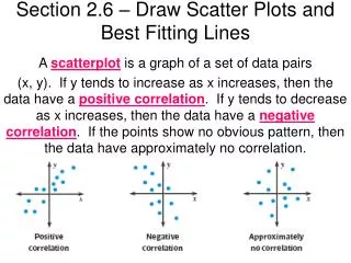
Scatter plot: A graph of a set of data pairs (x, y) Best-fitting line: the line that lies as close as possible to all the data points Median-median line: a linear model used to fit a line to a data set using summary points.
Describe the data as having a positive correlation, a negative correlation, or approximately no correlation. Tell whether the correlation coefficient for the data is closest to -1, -0.5, 0, 0.5, or 1. 1. 2. Positive Correlation correlation coefficient: 1 No Correlation correlation coefficient: 0
3. 4. Positive Correlation correlation coefficient: 0.5 Negative Correlation correlation coefficient: -1
5. The table below gives the number of people y who attended each of the first 7 football games x of the season. Approximate the best-fitting line for the data. Step 1: Draw a scatter plot
Step 2: Sketch the best fitting line. Step 3: Choose two points on the line. (1, 7) and (7, 1)
Step 4: Write an equation of the line that passes through the points. a. Find the slope. b. Use the point-slope form to write the equation. Remember: y = m(x – x1) + y1 y = -1(x – 1) + 7 y = -1x + 1 + 7 y = -x + 8
6. The table gives the average class score y on each unit test for the first six units x. Step 1: Draw a scatter plot
Step 2: Sketch the best fitting line. Step 3: Choose two points on the line. (3, 6) and (6, 10)
Step 4: Write an equation of the line that passes through the points. a. Find the slope. b. Use the point-slope form to write the equation.
7. Find the equation of the median-median line for the data. (1, 34), (2, 25), (3, 40), (5, 60), (6, 35), (7, 65), (9, 50), (10, 45), (11, 60) Step 1: Organize the data so that the x-values are in order from least to greatest. Then divided the coordinates into 3 equal sized groups. 1, 2, 3 34, 25, 40 5, 6, 7 60, 35, 65 9, 10, 11 50, 45, 60
Step 2: Find the median x-values and the median y-values for each group. 2 34 6 60 10 50 Step 3: Create a summary point for each group. Group 1: (____, ____) Group 2: (____, ____) Group 3: (____, ____) 2 34 6 60 10 50
Step 4: Determine the equation of the line between group 1 and 3. a. Find the slope: b. Use the point-slope form:
Step 5: Move the equation 1/3 of the way toward the middle summary point. middle summary point: (____, ____) predict value at x = ____ y = 2(____) + 30 = ____ one-third of the difference between y = ____ and y = ____ ⅓(60 – 42) ⅓(18) 6 Median-median line: y = 2x + 30 + 6 y = 2x+ 36 6 60 6 42 6 60 42
8. Find the equation of the median-median line for the data. (1, 25), (2, 20), (4, 35), (5, 43), (7, 53), (8, 40) (1.5, 22.5) (4.5, 39) (7.5, 46.5) y = 4(x – 1.5) + 22.5 y = 4x – 6 + 22.5 y = 4x + 16.5 y = 4(4.5) + 16.5 = 34.5 ⅓(39 – 34.5) = 1.5 y = 4x + 16.5 + 1.5 y = 4x + 18
(9). A histogram of the quiz grades for 46 students is pictured below. Estimate the mean and standard deviation for the data set.
Since the individual data elements are not given, both the mean and the standard deviation cannot be calculated exactly.
The data in the set is symmetrical, so the mean is the value in the center of the whole range, 0 to 25, which is 12.5.
Another method is to use the middle value of each bin as the representative for that bin. 12.5 7.5 17.5 22.5 2.5
Entering these values into our calculator, we find the mean is ________ and the standard deviation is _________. 12.72 5.61 12.5 7.5 17.5 22.5 2.5
(10). What is the range of possible means for the data set? We must first look at the least possible value for each bin and calculate the mean. 10 5 15 20 0 Mean = 10.22
Now, let’s look at the greatest possible value for each bin and calculate the mean. 15 10 20 25 5 Mean = 15.22
So the possible range of the means for this data set is 10.22 to 15.22.