Attribute Expression Using Gray Level Co-Occurrence

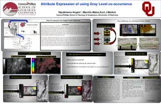
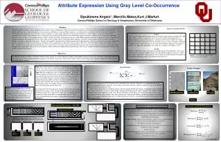
1. Attribute Expression Using Gray Level Co-Occurrence Gray level Gray level 7 7 0 0 Sipuikinene Angelo*, Marcilio Matos,Kurt J Marfurt ConocoPhillips School of Geology & Geophysics, University of Oklahoma 0 1 2 3 4 5 6 7 0 1 2 3 4 5 6 7 0 1 2 3 4 5 6 7 0 1 2 3 4 5 6 7 0 1 2 3 4 5 6 7 0 1 2 3 4 5 6 7 Summary Theory of Texture(GLCM) Seismic resolution remains a major limitation in the world of seismic interpretation. The goal of reflection seismology is to analyze seismic amplitude and character to predict lithologic facies, and rock properties such as porosity and thickness. Seismic attribute analysis is a technique that is commonly used by oil industry to delineate stratigraphic and structural features of interest. Seismic attributes, are particularly important in allowing the interpreter to extract subtlest at the limits below seismic resolution. For example, some attributes such as coherence and curvature are particularly good at identifying edges and fractures. Attributes such as spectral components tend to be more sensitive to stratigraphic thickness. Many commercial seismic interpretation packages contain RMS amplitude and relative impedance which is sensitive to acoustic impedance. My proposed research focuses upon seismic textural analysis, borrowing upon techniques commonly used in remote sensing to enhance and detect terrain, vegetation, and land use information. Textures are frequently characterized as different patterns in the underlying data. Seismic texture analysis was first introduced by Love and Simaan (1984) to extract patterns of common seismic signal character .Recently, several workers (West et al., 2002; Gao,2003; Chopra and Vladimir, 2005) have extended this technique to seismic through the uses of gray-level co-occurrence matrices(GLCM).The gray level, allows the recognition of patterns significantly more complex than simple edges. This set of texture attributes, is able to delineate complicated geological features such as mass complex transport and amalgamated channels that exhibit a distinct lateral pattern. Texture Texture is an everyday term relating to touch, that includes such concepts as rough, silky, and bumpy. When a texture is rough to the touch, the surface exhibits sharp differences in elevation within the space of your fingertip. In contrast, silky textures exhibit very small differences in elevation. Seismic textures work in the same way, except, elevation is replaced by brightness values (also called gray levels ). Instead of probing a finger over the surface, a "window" or a square box defining the size of the area, a probe is used (Halley, 2007) GLCM GLCM, is a tabulation of how often different combinations of Voxel brightness values (gray levels) occur in a sub-image window. In this research, GLCM compares a series of "second order" texture calculations, which quantifies and considers the relationship between groups of two (usually neighboring) pixels in the original image Figure 2b. Objectives Figure 1. A (5x5) GLCM matrices with its neighboring and reference pixel The objective of this research is to evaluate modern texture analysis as a tool to delineate complex Stratigraphic packages that are easy to identify, but perhaps difficult to map. This analysis will be based on pattern recognition and will be essential for features that exhibit a distinct lateral patter: mass transport complex ,dewatering features, and amalgamated channels . Gray level 05 Operational Processes - GLCM Figure 2a is characterized as a value of 1 corresponding to a trough a value of 3 to a zero crossing, and of 5 to a peak. A representative, (55) patch of seismic data using the discretization technique mentioned above. Figure 2b is the resulting gray-level co-occurrence matrix. Each row i, column j element of the gray-level co-occurrence matrix, indicates how many times the pixel lies to the right of the one value being analyzed. Texture calculations require a symmetrical matrix to account for the reciprocal nature of neighbor relations. To obtain symmetric matrices from the above definition, the resulting GLCM matrices are transposed. For 2D horizon slices, we compute the gray-level co-occurrence matrix in either 4 or 8 directions and sum the results. After making the GLCM symmetrical, there is still one more step to take before texture measures can be calculated. The measures require that each GLCM cell contain, not a count of how many times a combination pixel occurred, but rather a probability or normalization function. This is achieved by normalizing the matrices such that they each sum to 1.0 (see Equation 1). Normalization Texture Examples First step: Scale the data Sliding window GLCM 00 EQ = (1) Second step: Choose the direction, the offset, the size of the analysis window and calculate the GLCM matrix Equation one transforms the GLCM matrices into a probability mass function. Equation 1 is an approximation of the underlying probability density functions;. the true space of the image intensity values is continuous whereas the GLCM is being calculated using discrete values. Most texture calculations are weighted averages of the normalized GLCM cell contents. A weighted average multiplies each value to be used by a factor (a weight) before summing and dividing by the number of values. The weight is intended to express the relative importance of the value. When calculating a texture image, the result of the image will be a single value representing the entire window. This value is placed in the center of the window, and then the window is moved one pixel in the designated direction. This process is repeated and a new texture is calculated such that the entire image is built up of texture values. Figure 2. (a) A seismic trace scaled and biased to vary between 1 (a trough) and5 (a peak). Zero crossings have a value of 3. (b) A window of seismic data along a horizon slice. (c ) Resulting GLCM matrices and scale bar representing levels of intensity pixel occurrence. Random pattern Seismic Data Outcrop Contrast: 0 Correlation: 1.0000 Energy: 0.5102 Homogeneity: 1 Contrast: 49 Correlation: -1 Energy: 0.5000 Homogeneity: 0.1250 Contrast: 32.6667 Correlation: -0.5000 Energy: 0.3333 Homogeneity: 0.4167 Texture The more useful GLCM attributes Requirements for Human Interpretation To extract the key components of the GLCM , workers have formulated some 15 different texture measurements that can be calculated from the input GLCM. These measurements represent specific image properties such as contrast, orderliness and statistics. These three measurements are further subdivided into three groups. 1.Contrast Group: Measures are related to contrast ; it use weights related to the distance from the GLCM diagonal. Example: Dissimilarity, Contrast , Homogeneity 2.Orderliness Group: Orderliness means, how orderly the pixel values are within the window. Example: Entropy, Energy 3.Statistics Group: This third group of GLCM texture measures, consists of statistics derived from the GLC matrix. Example, Correlation, Variance 11/18/2008