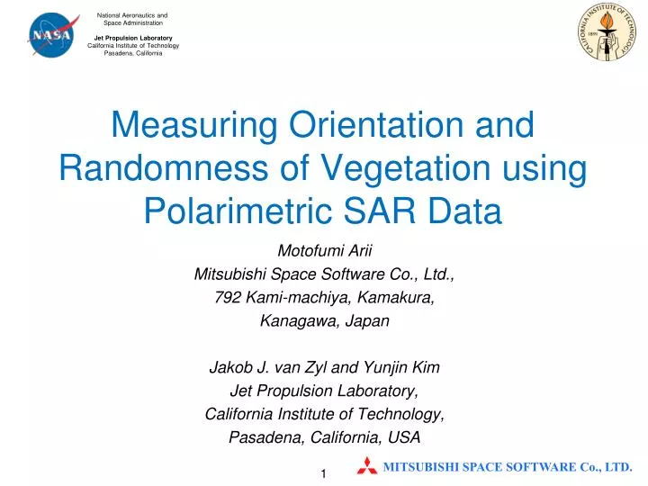
Measuring Orientation and Randomness of Vegetation using Polarimetric SAR Data

1. Measuring Orientation and Randomness of Vegetation using Polarimetric SAR Data Motofumi Arii Mitsubishi Space Software Co., Ltd., 792 Kami-machiya, Kamakura, Kanagawa, Japan Jakob J. van Zyl and Yunjin Kim Jet Propulsion Laboratory, California Institute of Technology, Pasadena, California, USA

2. Characterization of Volume Scattering Component We have modeledvegetation as a distribution of scattering elementswith several parameters. Mean orientation angle : Model Type of elementally scatterer : Randomness : a, b, c: complex number

3. Evolution of Volume Scattering Expression Freeman et al.[1] Yamaguchi et al. [2] Neumann et al. [3] Arii et al. [4] Type of elementally scatterer : S Uniform or medium Randomness : s Uniform any any Mean orientation angle : q0 None 0 or 90 any any a, b, c: complex number Flexibility [1] A. Freeman and S. L. Durden, “A three-component scattering model for polarimetric SAR data,” IEEE Trans. Geosci. Remote Sens., vol. 36, no. 3, pp. 964–973, May 1998. [2] Y. Yamaguchi, T. Moriyama, M. Ishido, and H. Yamada, “Fourcomponent scattering model for polarimetric SAR image decomposition,” IEEE Trans. Geosci. Remote Sens., vol. 43, no. 8, pp. 1699–1706, Aug. 2005. [3] M. Neumann, “Remote sensing of vegetation using multi-baseline polarimetric SAR interferometry: Theoretical modeling and physical parameter retrieval,” Ph.D. dissertation, Univ. Rennes, Rennes, France, 2009. [4] M. Arii, J. J. van Zyl, and Y. Kim, “A general characterization for polarimetric scattering from vegetation canopies,” IEEE Trans. Geosci. Remote Sens., vol. 48, no. 9, pp. 3349–3357, Sep. 2010.

4. Volume Component in the Polarimetric Decomposition Double-bounce Volume Surface Order of the estimation*1 First Second/Third Second/Third Degree of Freedom High Low Low possibly dominant error source In this presentation, we shall study the contribution of these vegetation parametersto the model-based polarimetric decomposition based on physical interpretation using Arii et al.’s general volume component and Non-negative eigenvalue decomposition (NNED)[5]. (*1) The order here is determined among volume, double-bounce and surface scattering from [1][2][4]. Other element such as helix in [2] is not taken into account. [5] J. J. van Zyl, M. Arii, and Y. Kim, “Model-based decomposition of polarimetric SAR covariance matrices constrained for nonnegative eigenvalues,” IEEE Trans. Geosci. Remote Sens., to be published.

5. Definition of Randomness and Orientation Large s =0.91 Uniform dist. Cosine squared dist. s q0 Randomness, s A : Normalization factor Delta function dist. q0 Small s =0

6. Arii et al.’s GeneralizedVolume Component[4]

7. Adaptive Model-Based Decomposition[6] Our observation can be decomposed as The form is slightly changed by simple transposition of terms. We estimate unknown parameters (S, q0, and s) by minimizing the reminder term. To achieve this, we firstly determine volume component, and then do the eigen value decomposition. [6] M. Arii, J. J. van Zyl, and Y. Kim, “Adaptive model-based decomposition of polarimetric SAR covariance matrices,” IEEE Trans. Geosci. Remote Sens., vol. 49, no. 3, pp. 1104–1113, Mar. 2011.

8. Black Forest Snapshot Forest A (38) Forest B (47) Forest C (57) Cropland (53) Forest D (63) Urban (59) L-band image of the Black Forest in Germany obtained by NASA/JPL AIRSAR system in the summer of 1991. The dotted arrows specify the direction of topographic change. Incidence angle for each area surrounded by solid rectangular is shown in the parentheses in degree.

9. Randomness and Entropy C-band L-band P-band suniform scos_sq s sdelta 1 H(s,S) 0

10. Definition of |a| and f By letting c=0 in the scattering matrix, scattering matrix for cylinder can be defined as where the a can be generally expressed as |a| and f are independent parameters.

11. |a| - f Zone Map Isotropic zone Double-bounce zone Dipole zone |a| - f zone map implicitly tells that the dipole can be a best candidate to represent volume scattering in the model-based decomposition because it is the furthermost from two other distinctive scatterers; isotropic and double-bounce.

12. Quick Look : Randomness By varying |a| and f, we can derive s and q0 as shown below. Forest A Forest B Forest C Forest D Urban Cropland C L P Double-bounce zone in urban area is significantly wider than that in the other areas as expected.

13. Quick Look : Mean Orientation Angle Double-bounce scattering Surface scattering Urban Cropland Forest A Forest B Forest C Forest D C L P Reddish pixels are recognized at L- and P-bands. These forested areas are more or less affected by double-bounce scattering at longer wavelengths due to the permeability of tree. Vertical Horizontal

14. Review of Surface and Double-Bounce Scattering To conduct further analysis, co-polarization ratio (HH/VV) of covariance matrix, Cv, derived from estimated s and f shall be used, where an effect of the order of decomposition should be significant. The a is fixed to zero (dipole) for simplicity. Before moving into the next step, following four facts will be quickly reviewed. • Fact A1: HH < VV for surface scattering • Fact A2 : Co-pol ratio for surface scattering decreases in terms of incidence angle • Fact B1 : HH > VV for double-bounce scattering • Fact B2 : Co-pol ratio for double-bounce scattering increases in terms of incidence angle

15. Fact A SPM [7] gives expressions for backscattering cross sections from rough surface as Then the ratio can be expressed as where Note that the ratio is a function of incidence angle and dielectric property. [7] S. O. Rice, “Reflection of electromagnetic waves from slightly rough surfaces,” Commun. Pure Appl. Math., vol. 4, pp. 351-378, 1951.

16. Fact A Simulated co-polarization ratio from rough surface in terms of incidence angle is shown in the figure. It can be easily recognized that the ratio is always less than one, i.e. HH<VV, and shows decreasing tendency in terms of incidence angle. Co-polarization ratio of ground scattering Incidence Angle (deg.)

17. Fact B1 Backscattering cross section of double-bounce scattering can be derived from Fresnel reflection coefficient. Flat Plate B BCS of double-bounce scattering [dB] Flat Plate A Incidence Angle (deg.) Brewster’s angle of Flat Plate B Brewster’s angle of Flat Plate A VV is generally smaller than HH due to Brewster’s angles for both flat plates.

18. Fact B2 With roughness on the ground, attenuation coefficient of specular scattering must be considerable.The coefficient [8] becomes Attenuated depending upon incidence angle Attenuation ratio, Catt Simulated attenuation coefficients at various bands are shown in the figure. For each case, increasing tendency is recognized in terms of incidence angle. Incidence Angle (deg.) [8] M. Arii, “Soil moisture retrieval under vegetation using polarimetric radar,” Ph.D. dissertation California Institute of Technology, Pasadena, CA, pp. 68-101, 2009.

19. Co-polarization Ratio in terms of Wavelength To investigate wavelength dependency, co-polarization ratios in terms of bands are plotted. The ratio for cropland stays around one whereas those for forestand urban are increasing. This follows our understanding, where scattering from agricultural area can be mainly contributed by surface scattering component (Fact A2), and that in urban is strongly affected by double-bounce scattering (Fact B) which should be dominant at longer wavelength due to its permeability. Co-polarization ratio 1 Wavelength (m)

20. Co-polarization Ratio in terms of Wavelength : Forest The ratio for each forest area is plotted. The ratios less than one are achieved for C-band, and they are increased as the wavelength increases. This is acceptable by considering attenuation effect which becomes significant with shorter wavelength. The increasing tendency at longer wavelengths would be mainly caused by horizontally oriented distributed branches or double-bounce scattering from Fact B. Co-polarization ratio 1 Wavelength (m)

21. Co-polarization Ratio in terms of Incidence Angle By comparing the C-band result with Fact A, shorter wavelength sees canopy as a rough surface. On the other hand, increasing tendencies at longer wavelengths may be explained by double-bounce scattering mechanism, or horizontally distributed volume scattering. Note that the P-band at higher incidence angle can penetrate volume layer more than L-band from Fact B2 so that it might be affected by another scattering mechanism such as azimuth tilt [5]. Co-polarization ratio Incidence Angle (deg.)

22. Summary and Future Work • We physically and quantitatively validated the adaptive model-based decomposition technique with fully generalized volume component for vegetation canopy. • We deepened our understanding of the behavior qualitatively based on co-polarization ratio in terms of incidence angles and frequencies. The ratio of the volume component shows significant sensitivity to the dominant scattering mechanism so that estimation error for each scattering mechanism is not negligible in some cases. For example, double-bounce scattering having HH>VV may be misinterpreted as higher amount of volume component with horizontal mean orientation angle. • Care must be paid when one applies the adaptive model-based decomposition with generalized volume component. Reasonable physical constraint based on solid understanding of scattering theory is now required. Sensitivity Study by Elaborated Forward Model Validation Fully Controlled Experiment