Download
1 / 36
370 likes | 558 Vues
(How best not to cool an LNA!). Aperture Array LNA Cooling. Is it economically viable (or even physically possible) to cool the tens of thousands of front-end LNAs used in an SKA aperture array station?. Presentation Overview: 1 – Aperture Array Review 2-PAD 2 – LNA Cooling Costing Model

E N D
(How best not to cool an LNA!) Aperture Array LNA Cooling Is it economically viable (or even physically possible) to cool the tens of thousands of front-end LNAs used in an SKA aperture array station? Presentation Overview: • 1 – Aperture Array Review • 2-PAD • 2 – LNA Cooling Costing Model • physics and features • results • 3 – LNA Cooling Measurement • description • results Presentation Overview
1000 SKA Reference Design 100 SKADS Benchmark 10 Field of View (deg2) 1 0.1 0.01 0.001 0.1 1 10 100 Frequency (GHz) SKADS Benchmark Scenario • Overall SKA concept • Low Frequency(0.1-0.3GHz)Sparse Apertura Array • Mid Frequency(0.3-1.0GHz)Dense Aperture Array • High Frequency(1.0-20GHz)Small Dishes • Aperture arrays are the only technology that provide survey speeds great enough to allow deep HI surveys • FoV = 250deg2 • Benchmark document available to download online at: • http://www.skads-eu.org/p/memos.php 1 – Aperture Array Review
Aperture Array Concept 1 – Aperture Array Review
Aperture Array Concept Look out for talk by:Georgina Harris 1 – Aperture Array Review
Aperture Array Electronics Front-end PCB • Look out for talks by: • Chris Shenton (digital), Tim Ikin (analogue) 1 – Aperture Array Review
Aperture Array Sensitivity • SKADS benchmark scenario document: • predicts the cost of an SKA aperture array station to be 3484k€ • assumes a Tsys of 50K for mid-frequency aperture array • a saving of 200k€ can be made if Tsys is reduced to 40K (§8.4) • Reducing Tsys • “Vital to get below 50K” Peter Wilkinson • Tsys might even be greater than 50K • future developments will see noise LNA decrease (14K from previous talk) • however cooling may still be required especially at high frequencies • cooling will also deliver temperature stabilisation 1 – Aperture Array Review
front-end PCB coax to antenna twisted pair to receiver cooling block cooling lines plastic casing plastic casing o-ring track cooling block hose fittings milled fluid channel Aperture Array LNA Cooling • Possible concept for cooling the front-end module using a metallic cooling block front-end PCB warmfluid out coldfluid in 1 – Aperture Array Review
Cooling Costing Model • The costing model / simulation code: • includes physics dealing with thermodynamics and hydrodynamics • costing includes: non-recurring expenses, replacement, electrical power • does not include: labour costs, no uncertainty analysis • written as a simple Matlab script (should be easy to convert, eg. Python) • might be able to become a ‘design block’ in the general SKA costing model • Assumptions / principle limitations • best estimates for input parameters used, some more inaccurate than others • chiller cost is assumed to be linearly proportional with power consumption, more costing ‘data points’ required to make a more accurate relationship • chiller cooling capacity efficiencies assumed to be equal for small and large chillers, more ‘real’ chiller specifications data are required • The Matlab script is currently available to download online at: • http://www.physics.ox.ac.uk/users/schediwy/cooling/ 2 – Cooling Costing Model
Cooling Costing Model • For the results in this presentation the code is configured to: • compare cost of a cooling system with the total cost SKA aperture array as specified in the SKADS Benchmark Scenario document (3500k€/station) • compare the power consumption with total station use (1000kW/station) • Three scenarios are compared: • 1 chiller located at the centre of the aperture array – “Model A” • 16 chillers distributed throughout the aperture array – “Model B” • 256 chiller distributed throughout the aperture array – “Model C” • The Matlab script is currently available to download online at: • http://www.physics.ox.ac.uk/users/schediwy/cooling/ 2 – Cooling Costing Model
Key: • chiller • pipe ‘D’ • pipe ‘C’ • pipe ‘B’ Cooling “Model A” • SKA aperture array station • Model A • chillers = 1 • pipe ‘D’ = 16 • pipe ‘C’ = 256 • pipe ‘B’ = 4096 • pipe ‘A’ = 65536 ~60m 2 – Cooling Costing Model
Key: • chiller • pipe ‘D’ • pipe ‘C’ • pipe ‘B’ Cooling “Model B” • SKA aperture array station • Model B • chillers = 16 • pipe ‘D’ = 0 • pipe ‘C’ = 256 • pipe ‘B’ = 4096 • pipe ‘A’ = 65536 ~60m 2 – Cooling Costing Model
Key: • chiller • pipe ‘D’ • pipe ‘C’ • pipe ‘B’ Cooling “Model C” • SKA aperture array station • Model C • chillers = 256 • pipe ‘D’ = 0 • pipe ‘C’ = 0 • pipe ‘B’ = 4096 • pipe ‘A’ = 65536 ~60m 2 – Cooling Costing Model
LNA cooling block Individual Component Heat Power Absorption Total System Heat Power Absorption pipe A pipe A pipe C pipe D pipe B total cooling capacity available from the chiller pipe A pipe B pipe B pipe C pipe C pipe D pipe D LNA cooling block pipe A pipe B pipe C pipe D Features – Heat Absorption • Assumed ambient temperature 30°C, desirable LNA temperature −20°C • Cooling much below this temperature is not possible with a glycol/water mixture • The chiller cooling capacity was adjusted to compensate for the total heat power absorbed by the cooling system • Insulation thickness was increased until the LNA was the dominant factor 2 – Cooling Costing Model
pipe C pipe D pipe B pipe A Total System Heat Power Absorption LNA cooling block pipe A pipe C pipe D pipe B total cooling capacity available from the chiller pipe A pipe B pipe C pipe D LNA cooling block pipe A pipe B pipe C pipe D Features – Heat Absorption • Assumed ambient temperature 30°C, desirable LNA temperature −20°C • Cooling much below this temperature is not possible with a glycol/water mixture • The chiller cooling capacity was adjusted to compensate for the total heat power absorbed by the cooling system • Insulation thickness was increased until the LNA was the dominant factor 2 – Cooling Costing Model
pipe ‘C’ext = 100mmint = 20mm pipe ‘D’external radius = 150mminternal radius = 50mm pipe ‘B’ext = 58.5mmint = 6.5mm pipe A0.82m3 pipe ‘A’ext = 34mmint = 2mm pipe B2.17m3 pipe D5.02m3 pipe C2.57m3 Features – Fluid Pipes • Pipe and insulation dimension: • Fluid volumes: 2 – Cooling Costing Model
pipe A pipe C pipe D pipe B LNA cooling block pipe A pipe D pipe D pipe C pipe B pipe D chiller pipe C pipe C LNA cooling block pipe B pipe B pipe A pipe A 0 1 2 3 4 5 6 7 8 9Position in Loop Features – Pressure/Flowrate • Chiller pressure must be great enough to drive fluid through cooling system • If there is too much pressure resistance the chiller flow rate will decrease • Flowrate was set so that Reynolds number is above 10,000 for all pipes • Dominated by inertial forces, viscous forces are minimised, turbulent flow 2 – Cooling Costing Model
Model A60.0k€ (1.7%) • Model B 51.1k€ (1.5%) • Model C44.0k€ (1.3%) 6.6k€ 17.5k€ 6.6k€ 6.6k€ 9.9k€ 17.0k€ 16.1k€ 9.9k€ 9.9k€ 7.4k€ 2.7k€ 14.1k€ 1.6k€ 7.4k€ 4.0k€ 7.4k€ 7.4k€ 2.7k€ Cooling Model Cost Results • All cooling models only cost a small fraction of the total aperture array • Model C results in the lowest price, mainly due to the reduction in coolant used • limitation: model currently does not take into account the difference in cooling efficiency (coefficient of performance) of different classes of chillers 2 – Cooling Costing Model
Electrical Power Consumption • Model A= 42.5kW × 1= 42.5kW • All models require only a small fraction (~4%) of the electrical power of the total aperture array (~1000kW) • Because of chiller assumption electrical power consumption of all models is very similar • Balance could change when chiller efficiencies are considered in detail • Model B= 2.57kW × 16= 41.1kW • Model C= 0.152kW × 256= 38.9W 2 – Cooling Costing Model
Cooling the LNA PCB • Close-up photo of the Avago LNA showing the cold finger in contact with the PCB thermocouple probe GaA LNA cold finger in contact with the PCB 3 – Experimental Cooling Work
Cooling the LNA PCB • The housing used to trap nitrogen to eliminate water condensation as the PCB warms-up to room temperature LNA PCB cold finger LN2 reservoir 50Ω terminator 3 – Experimental Cooling Work
LNA Noise Temperature • Plot of the broad-band noise temperature of the LNA PCB recorded at three different LNA temperatures (−50°C, −10°C and +30°C) 3 – Experimental Cooling Work
LNA Noise Temperature • Plot of LNA noise temperature of the LNA PCB at 700MHz measured at 17 different LNA temperatures 3 – Experimental Cooling Work
Conclusions / Further Work • Conclusions • cooling 10,000’s of LNA is not physically ridiculous • cooling could be economically beneficial • cost a small fraction of the full aperture array (<2%) • electrical power use is a small fraction of the full aperture array (~4%) • Further Work • only three models were studied in detail; further optimisation of parameter space may result in • more work required on some cost inputs, particularly chiller assumptions • presently work on low-loss potting compounds to minimise condensation problems • The Matlab script is currently available to download online at: • http://www.physics.ox.ac.uk/users/schediwy/cooling/ Conclusions
Questions? • The Matlab script is currently available to download online at: • http://www.physics.ox.ac.uk/users/schediwy/cooling/ Presentation End
Extra Slides 4 – Extra Slides
power supplies spectrum analyser 50Ω cold load copper coax gain chain v02 liquid nitrogen bath LNA Cooling Measurement • Photo of the experimental set-up used to measure the noise temperature of the LNA at various LNA temperatures 4 – Extra Slides
Physics Used in Model • Prandtl number • coolant specific heat • coolant dynamic viscosity • coolant thermal conductivity • Reynolds number • coolant density • coolant dynamic viscosity • coolant flow velocity • pipe hydrodynamic diameter • Hagen-Poiseuille Law • coolant volumetric flow rate • coolant dynamic viscosity • pipe length • pipe cross-sectional area • Heat transfer coefficient • coolant thermal conductivity • pipe Nusselt number • pipe hydrodynamic diameter • Dittus-Boelter correlation • Reynolds number • Prandtl number • Heat power absorbed • heat transfer coefficient • ambient temperature • coolant initial temperature • insulation thickness • insulation thermal conduction • pipe surface area 4 – Extra Slides
Current Limitations of Model • Insulation • Chiller flowrate large enough so that Reynolds number is above 10,000 for all pipes • means: flow is dominated by inertial forces, viscous forces are minimised, flow is turbulent • Cooling agents other than a glycol-water mixture would be too expensive, therefore minimum temperature limited to about −30°C • Incompressible fluid – very small effect • Laminar flow - • Wall friction – Darcy-Weisbach equation – easy to include in the future • Joint/Corner effects • Chiller efficiencies 4 – Extra Slides
3 Different Cooling Models • Schematic representation of three models investigated using a Matlab cooling and costing simulation pipe D pipe B pipe A pipe C x16 x16 x16 x16 antennapairs Model A1 central chiller chillers subtiles 1 16 256 4096 65536 large pipe small pipe x16 x16 x16 antennapairs Model B16 distributed chillers subtiles chillers 16 256 4096 65536 • The physical layout of three concepts are shown on the next slide large pipe small pipe x16 x16 antennapairs subtiles chillers Model C256 distributedchillers 256 4096 65536 4 – Extra Slides
3 4 Cascade Element: 1 2 50Ω Terminator Copper Coax Gain Chain v02 Spectrum Analyser Avago LNA Cascade Analysis • Factors affecting Tsys: • sky temperature • front-end LNA • rest of system 4 – Extra Slides
SKADS Station Data Flow 4 – Extra Slides
Nitrogen Atmosphere • A photo of the demo-board after warming back up to room temperature excess condensation collects on cold finger no condensation visible on PCB 4 – Extra Slides
LNA Temperature Increase LN2 evaporated Cold Finger Removed 4 – Extra Slides
Avago LNA – Testboard 1 4 – Extra Slides
Aperture Array Mounting 2.56m 4 – Extra Slides
~13mm ~4mm ~13mm ~13mm CAT 7 and Cooling 30 Leads ~35mm Low DensityPoly Pipe 13mm X 100M: A$43.02 CAT 7 37 Leads 37Leads ~13mm 4 – Extra Slides