Download
1 / 13

E N D
Quantifying data • Given a sample space, we are often interested in some numerical property of the outcomes. For example, if our collection is college students, we may be interested in their height. Or their weight or their IQ or any other property which we could somehow assign a number. • This is motivation for the idea of a random variable.
A random variable is a rule (like a function) that enables us to assign a number to each outcome of a sample space. The actual number associated with the outcome is called the value. • We distinguish between a discrete and continuous random variable.
Some examples • Suppose I have a collection of books, and I pick one book at random. Then my sample space is just that same collection of books. A discrete variable could be • The number of pages of the book. • The number of words in the book. • The number of pages of the last chapter. • 0 if the book does not contain a preface, 1 if the book does contain a preface. • 1 if the book is between 1 and 100 pages, 2 if the book is between 101 and 200 pages, etc.
Let’s look at an example in detail. I have 208 (math) books in my office. • Suppose I wish to organize them according to “area of math” i.e. my discrete variable is “area of math.” • Here is the breakdown: 28 algebra, 55 history, 20 number theory, 48 Calculus, 57 topology. • This is an example of a probability distribution.
The Idea • Consider our old go-to experiment of tossing a fair cone two times. The sample space S={HH, HT, TH, TT}. What is the probability of obtaining each event as an outcome? • Any event in the sample space has equal probability, 1/4, of being selected. There are 4 possible outcomes and so 1/4+1/4+1/4+1/4=1. This observation almost seems silly.
Suppose now that the coin is “weighted” with a 60% chance of landing on a head and a 40% chance of landing on a tail. We still have the same sample space, but now the probabilities are as follows: P(HH)=.36, P(TH)=P(HT)=.24, and P(TT)=.16. But again .36+.24+.24+.16=1. • We thus define the specifications of the probabilities associated with the various distinct values of a discrete random variable to be a discrete probability distribution. The probability associated with the value x is denoted P(x).
Examples • Consider the probability distribution • Find P(x=C) and P(x=E). • P(x=A or x=B). • In a general discrete distribution, P(x=a or x=b)=P(a)+P(b).
Probability Histograms • Here we plot each x value as a bar with height P(x). • For the data set • Construct a probability histogram. • This gives a good graphic way of displaying your probability distribution.
Practice Problem • The following shows the distribution of the number of misspellings in a 250 word essay. • Find P(x=2), P(x=1 or x=6), P(x<4), and P(x≤4). Construct a probability histogram.
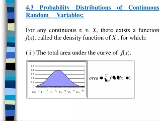
Discrete vs. Continuous • Consider the example above where our random variable is the number of pages of a book. It is certainly possible for the value of a particular book to be 243 or 244. But is it possible to be 243.11? • In contrast, consider a collection of the days of the year in 2008 in Collegeville, and let our random variable assign to each day the temperature on that particular day in Collegeville. Not only is it possible to obtain the values 53 and 54, but one could technically obtain the value 53.7, 53.78, 53.781, etc. depending on how accurate our instruments are, at least in theory. But there is no such thing as a book with one-quarter of a page. • This leads us to the following definition.
A random variable is said to be continuous if it can potentially take on any value in between any two points where the random variable is defined. A random variable is discrete if the values it can potentially assume a sequence of isolated points. • Examples: The sum of a roll of 4 dice. • Age in whole years. • Age as exact as possible at a certain point.
Normal Distributions Our old friend the normal distribution is an example of continuous probability distribution. For μ=10 and σ=2, find P(x<6), P(x>11 or x<4) and P(x≤6).