Random Variable Overview
Random Variable Overview. What are random variables? Intro to probability distributions Discrete Continuous Linear transformations of RVs Combinations of RVs. What are random variables?. Let X represent a quantitative variable that is measured or observed in an experiment.

Random Variable Overview
E N D
Presentation Transcript
Random Variable Overview • What are random variables? • Intro to probability distributions • Discrete • Continuous • Linear transformations of RVs • Combinations of RVs
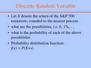
What are random variables? Let X represent a quantitative variable that is measured or observed in an experiment. The value that X takes on in a given experiment is a random outcome. • Counting the number of defective lightbulbs in a case of bulbs • Measuring daily rainfall in inches • Measuring the average depression score of computer science majors
Sample means, standard deviations, proportions, and frequencies are all random variables.
Two types of random variables Discrete Continuous The observations can take only a finite, countable number of values. The observations can take on any of the countless number of values in an interval • The number of heads in four coin tosses • The number of anorexics in a random sample of 500 people • The average response time of a random sample of 200 depressed patients • The average IQ of a random sample of 22 statistics students
In general, averages are continuous and counts are discrete. The average anger response The number of juvenile delinquents
Discrete Continuous The probabilities associated with each specific value of the RV The probabilities associated with a range of values of the RV. What is a probability distribution?
Two balls are randomly chosen from an urn of blue and red balls. We win $1 for every blue and lose $1 for every red. Let X = our total winnings. Suppose that we toss three coins. Let X = the number of heads appearing. X is a random variable taking on one of the values -2, 0, 2 X is a random variable taking on one of the values 0,1,2,3 The Sample Space
Suppose that we toss two dice. Let X = the difference of the two tosses. Suppose that we toss two dice. Let X = the sum of the two tosses. X is a random variable taking on one of the values ___________ X is a random variable taking on one of the values _________ The Sample Space
Suppose that we toss a fair die. Let X = the outcome of the toss. xi pi 1 1/6 2 1/6 3 1/6 4 1/6 5 1/6 6 1/6 X is a random variable taking on one of the values 1, 2, 3, 4, 5, 6 Probability Distributions The probability distribution of X lists the values in the sample space and their associated probabilities.
xi pi 1 1/6 2 1/6 3 1/6 4 1/6 5 1/6 6 1/6 probability outcome Probability Distributions The probability distribution of X lists the values in the sample space and their associated probabilities.
Probability Distributions Suppose that we toss two coins. Let X = the number of heads. Make the probability distribution
xi pi 0 1/4 1 2/4 2 1/4 probability outcome Probability Distributions Suppose that we toss two coins. Let X = the number of heads. Make the probability distribution
xi pi A 73/1000 B 9/1000 C 30/1000 D 44/1000 E 130/1000 F 28/1000 probability outcome Probability Distributions Sometimes you can estimate discrete probability distributions using a really large sample Cryptography: Frequencies of letters in a 1000 letter sample
Expected Values The mean of a discrete probability distribution (called the “expected value”) can be found using this formula It is a weighted average of the possible values of X, each value being weighted by its probability of occurrence.
xi pi 1 1/6 2 1/6 3 1/6 4 1/6 5 1/6 6 1/6 Suppose that we toss a fair die. Let X = the outcome of the toss. X is a random variable taking on one of the values 1, 2, 3, 4, 5, 6 Expected Values What is the expected value?
xi pi Expected Values Suppose we draw one marble out of a bowl containing 3 green and 7 black marbles. We win $10 if we draw a green marble but we lose $2 if we draw a black marble. Let X = our winnings. What is the expected value of X? Should you play this game? 3/10 7/10 10 -2
Variance The variance of a discrete probability distribution can be found using this formula It is a weighted average of the squared deviations in X
xi pi 1 1/6 2 1/6 3 1/6 4 1/6 5 1/6 6 1/6 Suppose that we toss a fair die. Let X = the outcome of the toss. X is a random variable taking on one of the values 1, 2, 3, 4, 5, 6 • μx = 3.5 • σx2 = ?
xi pi (xi-X)2 1 1/6 6.25 2 1/6 2.25 3 1/6 .25 4 1/6 .25 5 1/6 2.25 6 1/6 6.25 Suppose that we toss a fair die. Let X = the outcome of the toss. X is a random variable taking on one of the values 1, 2, 3, 4, 5, 6 • μx = 3.5 • σx2 = ?
xi pi (xi-X)2 Suppose that we toss a coin. Let X = 1 if it’s heads and 0 if it’s tails. What is the expected value of X? What is the variance? μ = .50 σ2 = .25
xi pi (xi-X)2 Suppose that we toss 3 coins. For every head we get $1 and for every tail we lose $1. Let X = our winnings. What is the expected value of X? What is the variance of X? μ = 0 σ2 = 3
Known Discrete Distributions • The bernoulli (heads versus tails) • The binomial (# heads in n tosses) • The poisson (# customers entering a post office in a day)
Continuous Probability Distributions • We talk about probabilities for a range of values, not a particular value. • Probability for a range of values is determined by the area under the probability distribution curve (use calculus or a table). • Expected value Variance
Known Continuous Distributions • The uniform distribution • The normal distribution • The t distribution • The F distribution
The probability distribution curve for the normal distribution N(µ,σ) is defined by this function • Luckily, you can you can find the probabilities for this curve using Table E • Expected value Variance Normal Distribution
Standard Normal Distribution • A normal distribution has mean μx and variance σx2 • The standard normal distribution is a normal distribution that has been transformed to have mean 0 and variance 1 • If raw scores are normally distributed, the distribution of z-scores will be standard normal • Thus if raw scores are normally distributed, we can associate z-scores with standard normal probabilities • (whether or not raw scores are normally distributed, a z-score accurately indexes/positions a score in terms of the number of standard deviations away from the mean)
Interpreting Z Scores Unusual Values Ordinary Values Unusual Values - 3 - 2 - 1 0 1 2 3 Z
Z-scores: Handy for thinking about the normal probability distribution • If the distribution of raw scores is normal, the z distribution will be “standard normal” Z scores • This is a probability density curve • In particular, it is the “standard normal” probability distribution • Probability corresponds to area under the curve • Total area under the curve is 1
Area = 0.3413 • 1 standard deviation includes about 68% of cases (34% on each side) • 2 standard deviations includes about 95% of cases • 3 standard deviations includes about 99.7% of cases Standard Normal Distribution Z scores ASSUMING RAW SCORES DISTRIBUTED NORMALLY
Using Appendix E.10 • For positive z scores, gives you area under curve that corresponds to probability • For negative z scores, use the complement rule z z z μ μ μ z mean to larger smaller z portion portion .00 0.0000 0.5000 0.5000 .50 0.1915 0.6915 0.3085 1.0 0.3413 0.8413 0.1587 1.5 0.4332 0.9332 0.0668 2.0 0.4772 0.9772 0.0228 2.5 0.4938 0.9938 0.0062
? ? 0.4429 -3 -2 -1 0 1 2 3 0.0571 1.58 0 Score (z ) Standard Normal Distribution Area found in Appx E.10 Area = 0.3413 Area = 0.1587 Score (z )
Exercise What is the probability of getting a Z greater than 1.96? What z-score will give you a probability of 5% in the upper tail?
Applications Let’s say the population of bartenders has an IQ of 100 and a standard deviation of 10 If we measure the IQ of any one bartender, how likely is it that her score would be greater than 80?
P(x > 80) = ? Step 1: Translate the score into z score Step 2: Use E.10 to get probability P(Z > -2) = 98%
Exercise Let’s say the population of bartenders has an IQ of 100 and a standard deviation of 10 If we measure the IQ of any one bartender, how likely is it that her score would be Greater than 80? Between 90 and 110? Greater than 115?
Rules for Expected Values Linear Transformations: If you add/subtract a constant to the RV, then add/subtract that number to the X If you mult/divide the RV by a constant, then mult/divide the X by that number Combining Two Random Variables If you add random variable X to random variable Y, then add X to Y If you subtractrandom variable X from random variable Y, then subtract X from Y
Rules for Variances of Random Variables Linear Transformations: If you add/subtract a constant to the RV, then nothing happens to X2 If you mult/divide the RV by a constant, then mult/divide the X2 by that number squared Combining Two Independent Random Variables If you add random variable X to random variable Y, then add X2 to Y2 If you subtract random variable X from random variable Y, then add X2 to Y2
Example 1 Suppose that we toss a coin. Let X = 1 if it’s heads and 0 if it’s tails. What is the expected value of X? X = ______ What is the variance of X? σx2 = _____ Now we go into a special “double or nothing” round. All dollar values are doubled in this round. What is the new expected value of X? x = ______ What is the new variance of X? σx2 = _____ .50 1.00 .25 1.00
Example 2 Suppose that we toss a coin. Let X = 1 if it’s heads and 0 if it’s tails. What is the expected value of X? X = ______ What is the variance of X? σx2 = _____ Now suppose we toss three coins. What is the expected value of all three tosses combined? X+Y+Z = ______ What is the new variance? σX+Y+Z = _____ .50 1.50 .25 .75
Example 3 50 vegetarians and 100 non-vegetarians participate in a study of cardiovascular health. On average, the vegetarians received a score of 80 with a standard deviation of 5. The non-vegetarians scored 70 points on average with a standard deviation of 10. A sneaky researcher tries to fudge the data by multiplying the scores of the non-vegetarians by 1.2 and adding 5 points. What happens to the mean and sd?
Example 4 100 pairs of male-female siblings participate in a study of repressive coping. For the women, the average repressive coping score was 6 with a standard deviation of .5. For men, the average repressive coping score was 5, with a standard deviation of .5. What is the average and standard deviation of the set of male-female difference scores?