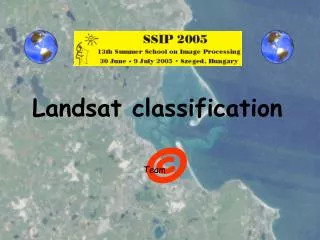
Landsat classification
Landsat classification. ©. Team. ©. Team. Delia Mitrea – Technical University of Cluj-Napoca, Romania Sándor Szolyka – Budapest Tech, Hungary Imre Hajagos – University of Szeged, Hungary Szabolcs Berecz - Budapest Tech, Hungary

Landsat classification
E N D
Presentation Transcript
Landsat classification © Team
© Team Delia Mitrea – Technical University of Cluj-Napoca, Romania Sándor Szolyka – Budapest Tech, Hungary Imre Hajagos – University of Szeged, Hungary Szabolcs Berecz - Budapest Tech, Hungary Gergely Grósz – University of Veszprém Georgikon Faculty of Agricultural, Hungary SSIP 2005
The Problem • Input: Landsat images of terrain, plus sample images of fields, sea, forests or etc. • Aim: Segmentation of scene based on texture and colour. • Output: Label scene. SSIP 2005
The Solution Solution 1. - Histogram matching I. Step 1. Decompose the image into small cells. Step 2. Compute the histogram in the RGB levels (All grid has three (red, green, blue) histograms.). Step 3. Classification based on the correlation of histograms. Step 4. Segment the image. SSIP 2005
The Solution SSIP 2005
The Solution Solution 2. - Histogram matching II. Convert the histograms to a greyscale. (Y=0,299 R+0,587 G+0,114 B) SSIP 2005
The Solution Solution 3. – Markov Random Fields • Statistics based classifier algorithm. • Uses spatial information. • Driven by energy minimization. SSIP 2005
The Solution Solution 4. - Texture-based recognition • Features used: • Average edge frequency (density) • Average edge contrast • GLCM (Gray Level Cooccurrence Matrix) homogeneity • GLCM (Gray Level Cooccurrence Matrix) entropy • GLCM (Gray Level Cooccurrence Matrix) variance • GLCM (Gray Level Cooccurrence Matrix) energy SSIP 2005
The Solution Solution 4. - Texture-based recognition Step 1. Learning • Select a known region int the image (forest mountains or water) • Compute GLCM features and edge-based features • Store the feature vector in the training set for the corresponding class SSIP 2005
The Solution Solution 4. - Texture-based recognition Step 2. Recognition • Select an unknown area in the image in order to classify it: forest mountains or water • Compute the GLCM features and the edge-based features • Compare the feature vectors with the data int he training set: euclidean distance • Use the k-nn method and decide the class SSIP 2005
The Solution Solution 4. - Texture-based recognition SSIP 2005
References • M. Berthod, Z. Kato, S. Yu, J. Zerubia: Bayesian imageclassification using Markov random fields. Image and Vision Computing,14(1996): 285-295, 1996. • Z. Kato: Multi-scale Markovian Modelisation in Computer Vision withApplications to SPOT Image Segmentation. PhD thesis, INRIA SophiaAntipolis, France, 1994. • Z. Kato, J. Zerubia and M. Berthod: Satellite image classification using amodified Metropolis dynamics Proc. IEEE International Conf. on Acoust., Speechand Sig. Proc., vol. 3, pp. 573-576, San Francisco, CA, March 23-26,1992. SSIP 2005
The End Thank you for your attention!