Download
1 / 48
490 likes | 1.94k Vues
t TEST OF A HYPOTHESIS RELATING TO A REGRESSION COEFFICIENT s.d. of b 2 known discrepancy between hypothetical value and sample estimate, in terms of s.d.: 5% significance test: reject H 0 : b 2 = b 2 if z > 1.96 or z < – 1.96 0

E N D
t TEST OF A HYPOTHESIS RELATING TO A REGRESSION COEFFICIENT s.d. of b2 known discrepancy between hypothetical value and sample estimate, in terms of s.d.: 5% significance test: reject H0: b2 = b2 if z > 1.96 or z < –1.96 0 The diagram summarizes the procedure for performing a 5% significance test on the slope coefficient of a regression under the assumption that we know its standard deviation. 1
t TEST OF A HYPOTHESIS RELATING TO A REGRESSION COEFFICIENT s.d. of b2 known s.d. of b2 not known discrepancy between hypothetical value and sample estimate, in terms of s.d.: discrepancy between hypothetical value and sample estimate, in terms of s.e.: 5% significance test: reject H0: b2 = b2 if z > 1.96 or z < –1.96 0 This is a very unrealistic assumption. We usually have to estimate it with the standard error, and we use this in the test statistic instead of the standard deviation. 2
t TEST OF A HYPOTHESIS RELATING TO A REGRESSION COEFFICIENT s.d. of b2 known s.d. of b2 not known discrepancy between hypothetical value and sample estimate, in terms of s.d.: discrepancy between hypothetical value and sample estimate, in terms of s.e.: 5% significance test: reject H0: b2 = b2 if z > 1.96 or z < –1.96 0 Because we have replaced the standard deviation in its denominator with the standard error, the test statistic has a t distribution instead of a normal distribution. 3
t TEST OF A HYPOTHESIS RELATING TO A REGRESSION COEFFICIENT s.d. of b2 known s.d. of b2 not known discrepancy between hypothetical value and sample estimate, in terms of s.d.: discrepancy between hypothetical value and sample estimate, in terms of s.e.: 5% significance test: reject H0: b2 = b2 if z > 1.96 or z < –1.96 5% significance test: reject H0: b2 = b2 if t > tcrit or t < –tcrit 0 0 Accordingly, we refer to the test statistic as a t statistic. In other respects the test procedure is much the same. 4
t TEST OF A HYPOTHESIS RELATING TO A REGRESSION COEFFICIENT s.d. of b2 known s.d. of b2 not known discrepancy between hypothetical value and sample estimate, in terms of s.d.: discrepancy between hypothetical value and sample estimate, in terms of s.e.: 5% significance test: reject H0: b2 = b2 if z > 1.96 or z < –1.96 5% significance test: reject H0: b2 = b2 if t > tcrit or t < –tcrit 0 0 We look up the critical value of t and if the t statistic is greater than it, positive or negative, we reject the null hypothesis. If it is not, we do not. 5
t TEST OF A HYPOTHESIS RELATING TO A REGRESSION COEFFICIENT normal Here is a graph of a normal distribution with zero mean and unit variance 6
t TEST OF A HYPOTHESIS RELATING TO A REGRESSION COEFFICIENT normal t, 10 d.f. A graph of a t distribution with 10 degrees of freedom (this term will be defined in a moment) has been added. 7
t TEST OF A HYPOTHESIS RELATING TO A REGRESSION COEFFICIENT normal t, 10 d.f. When the number of degrees of freedom is large, the t distribution looks very much like a normal distribution (and as the number increases, it converges on one). 8
t TEST OF A HYPOTHESIS RELATING TO A REGRESSION COEFFICIENT normal t, 10 d.f. Even when the number of degrees of freedom is small, as in this case, the distributions are very similar. 9
t TEST OF A HYPOTHESIS RELATING TO A REGRESSION COEFFICIENT normal t, 10 d.f. t, 5 d.f. Here is another t distribution, this time with only 5 degrees of freedom. It is still very similar to a normal distribution. 10
t TEST OF A HYPOTHESIS RELATING TO A REGRESSION COEFFICIENT normal t, 10 d.f. t, 5 d.f. So why do we make such a fuss about referring to the t distribution rather than the normal distribution? Would it really matter if we always used 1.96 for the 5% test and 2.58 for the 1% test? 11
t TEST OF A HYPOTHESIS RELATING TO A REGRESSION COEFFICIENT normal t, 10 d.f. t, 5 d.f. The answer is that it does make a difference. Although the distributions are generally quite similar, the t distribution has longer tails than the normal distribution, the difference being the greater, the smaller the number of degrees of freedom. 12
t TEST OF A HYPOTHESIS RELATING TO A REGRESSION COEFFICIENT normal t, 10 d.f. t, 5 d.f. As a consequence, the probability of obtaining a high test statistic on a pure chance basis is greater with a t distribution than with a normal distribution. 13
t TEST OF A HYPOTHESIS RELATING TO A REGRESSION COEFFICIENT normal t, 10 d.f. t, 5 d.f. This means that the rejection regions have to start more standard deviations away from zero for a t distribution than for a normal distribution. 14
t TEST OF A HYPOTHESIS RELATING TO A REGRESSION COEFFICIENT normal t, 10 d.f. t, 5 d.f. -1.96 The 2.5% tail of a normal distribution starts 1.96 standard deviations from its mean. 15
t TEST OF A HYPOTHESIS RELATING TO A REGRESSION COEFFICIENT normal t, 10 d.f. t, 5 d.f. -2.33 The 2.5% tail of a t distribution with 10 degrees of freedom starts 2.33 standard deviations from its mean. 16
t TEST OF A HYPOTHESIS RELATING TO A REGRESSION COEFFICIENT normal t, 10 d.f. t, 5 d.f. -2.57 That for a t distribution with 5 degrees of freedom starts 2.57 standard deviations from its mean. 17
t TEST OF A HYPOTHESIS RELATING TO A REGRESSION COEFFICIENT t Distribution: Critical values of t Degrees of Two-sided test 10% 5% 2% 1% 0.2% 0.1% freedom One-sided test 5% 2.5% 1% 0.5% 0.1% 0.05% 1 6.314 12.706 31.821 63.657 318.31 636.62 2 2.920 4.303 6.965 9.925 22.327 31.598 3 2.353 3.182 4.541 5.841 10.214 12.924 4 2.132 2.776 3.747 4.604 7.173 8.610 5 2.015 2.571 3.365 4.032 5.893 6.869 … … … … … … … … … … … … … … 18 1.734 2.101 2.552 2.878 3.610 3.922 19 1.729 2.093 2.539 2.861 3.579 3.883 20 1.725 2.086 2.528 2.845 3.552 3.850 … … … … … … … … … … … … … … 600 1.647 1.964 2.333 2.584 3.104 3.307 1.645 1.960 2.326 2.576 3.090 3.291 For this reason we need to refer to a table of critical values of t when performing significance tests on the coefficients of a regression equation. 18
t TEST OF A HYPOTHESIS RELATING TO A REGRESSION COEFFICIENT t Distribution: Critical values of t Degrees of Two-sided test 10% 5% 2% 1% 0.2% 0.1% freedom One-sided test 5% 2.5% 1% 0.5% 0.1% 0.05% 1 6.314 12.706 31.821 63.657 318.31 636.62 2 2.920 4.303 6.965 9.925 22.327 31.598 3 2.353 3.182 4.541 5.841 10.214 12.924 4 2.132 2.776 3.747 4.604 7.173 8.610 5 2.015 2.571 3.365 4.032 5.893 6.869 … … … … … … … … … … … … … … 18 1.734 2.101 2.552 2.878 3.610 3.922 19 1.729 2.093 2.539 2.861 3.579 3.883 20 1.725 2.086 2.528 2.845 3.552 3.850 … … … … … … … … … … … … … … 600 1.647 1.964 2.333 2.584 3.104 3.307 1.645 1.960 2.326 2.576 3.090 3.291 At the top of the table are listed possible significance levels for a test. For the time being we will be performing two-sided tests, so ignore the line for one-sided tests. 19
t TEST OF A HYPOTHESIS RELATING TO A REGRESSION COEFFICIENT t Distribution: Critical values of t Degrees of Two-sided test 10% 5% 2% 1% 0.2% 0.1% freedom One-sided test 5% 2.5% 1% 0.5% 0.1% 0.05% 1 6.314 12.706 31.821 63.657 318.31 636.62 2 2.920 4.303 6.965 9.925 22.327 31.598 3 2.353 3.182 4.541 5.841 10.214 12.924 4 2.132 2.776 3.747 4.604 7.173 8.610 5 2.015 2.571 3.365 4.032 5.893 6.869 … … … … … … … … … … … … … … 18 1.734 2.101 2.552 2.878 3.610 3.922 19 1.729 2.093 2.539 2.861 3.579 3.883 20 1.725 2.086 2.528 2.845 3.552 3.850 … … … … … … … … … … … … … … 600 1.647 1.964 2.333 2.584 3.104 3.307 1.645 1.960 2.326 2.576 3.090 3.291 Hence if we are performing a (two-sided) 5% significance test, we should use the column thus indicated in the table. 20
t TEST OF A HYPOTHESIS RELATING TO A REGRESSION COEFFICIENT t Distribution: Critical values of t Degrees of Two-sided test 10% 5% 2% 1% 0.2% 0.1% freedom One-sided test 5% 2.5% 1% 0.5% 0.1% 0.05% 1 6.314 12.706 31.821 63.657 318.31 636.62 2 2.920 4.303 6.965 9.925 22.327 31.598 3 2.353 3.182 4.541 5.841 10.214 12.924 4 2.132 2.776 3.747 4.604 7.173 8.610 5 2.015 2.571 3.365 4.032 5.893 6.869 … … … … … … … … … … … … … … 18 1.734 2.101 2.552 2.878 3.610 3.922 19 1.729 2.093 2.539 2.861 3.579 3.883 20 1.725 2.086 2.528 2.845 3.552 3.850 … … … … … … … … … … … … … … 600 1.647 1.964 2.333 2.584 3.104 3.307 1.645 1.960 2.326 2.576 3.090 3.291 Number of degrees of freedom in a regression = number of observations – number of parameters estimated. The left hand vertical column lists degrees of freedom. The number of degrees of freedom in a regression is defined to be the number of observations minus the number of parameters estimated. 21
t TEST OF A HYPOTHESIS RELATING TO A REGRESSION COEFFICIENT t Distribution: Critical values of t Degrees of Two-sided test 10% 5% 2% 1% 0.2% 0.1% freedom One-sided test 5% 2.5% 1% 0.5% 0.1% 0.05% 1 6.314 12.706 31.821 63.657 318.31 636.62 2 2.920 4.303 6.965 9.925 22.327 31.598 3 2.353 3.182 4.541 5.841 10.214 12.924 4 2.132 2.776 3.747 4.604 7.173 8.610 5 2.015 2.571 3.365 4.032 5.893 6.869 … … … … … … … … … … … … … … 18 1.734 2.101 2.552 2.878 3.610 3.922 19 1.729 2.093 2.539 2.861 3.579 3.883 20 1.725 2.086 2.528 2.845 3.552 3.850 … … … … … … … … … … … … … … 600 1.647 1.964 2.333 2.584 3.104 3.307 1.645 1.960 2.326 2.576 3.090 3.291 In a simple regression, we estimate just two parameters, the constant and the slope coefficient, so the number of degrees of freedom is n - 2 if there are n observations. 22
t TEST OF A HYPOTHESIS RELATING TO A REGRESSION COEFFICIENT t Distribution: Critical values of t Degrees of Two-sided test 10% 5% 2% 1% 0.2% 0.1% freedom One-sided test 5% 2.5% 1% 0.5% 0.1% 0.05% 1 6.314 12.706 31.821 63.657 318.31 636.62 2 2.920 4.303 6.965 9.925 22.327 31.598 3 2.353 3.182 4.541 5.841 10.214 12.924 4 2.132 2.776 3.747 4.604 7.173 8.610 5 2.015 2.571 3.365 4.032 5.893 6.869 … … … … … … … … … … … … … … 18 1.734 2.101 2.552 2.878 3.610 3.922 19 1.729 2.093 2.539 2.861 3.579 3.883 20 1.725 2.086 2.528 2.845 3.552 3.850 … … … … … … … … … … … … … … 600 1.647 1.964 2.333 2.584 3.104 3.307 1.645 1.960 2.326 2.576 3.090 3.291 If we were performing a regression with 20 observations, as in the price inflation/wage inflation example, the number of degrees of freedom would be 18 and the critical value of t for a 5% test would be 2.101. 23
t TEST OF A HYPOTHESIS RELATING TO A REGRESSION COEFFICIENT t Distribution: Critical values of t Degrees of Two-sided test 10% 5% 2% 1% 0.2% 0.1% freedom One-sided test 5% 2.5% 1% 0.5% 0.1% 0.05% 1 6.314 12.706 31.821 63.657 318.31 636.62 2 2.920 4.303 6.965 9.925 22.327 31.598 3 2.353 3.182 4.541 5.841 10.214 12.924 4 2.132 2.776 3.747 4.604 7.173 8.610 5 2.015 2.571 3.365 4.032 5.893 6.869 … … … … … … … … … … … … … … 18 1.734 2.101 2.552 2.878 3.610 3.922 19 1.729 2.093 2.539 2.861 3.579 3.883 20 1.725 2.086 2.528 2.845 3.552 3.850 … … … … … … … … … … … … … … 600 1.647 1.964 2.333 2.584 3.104 3.307 1.645 1.960 2.326 2.576 3.090 3.291 Note that as the number of degrees of freedom becomes large, the critical value converges on 1.96, the critical value for the normal distribution. This is because the t distribution converges on the normal distribution. 24
t TEST OF A HYPOTHESIS RELATING TO A REGRESSION COEFFICIENT s.d. of b2 known s.d. of b2 not known discrepancy between hypothetical value and sample estimate, in terms of s.d.: discrepancy between hypothetical value and sample estimate, in terms of s.e.: 5% significance test: reject H0: b2 = b2 if z > 1.96 or z < –1.96 5% significance test: reject H0: b2 = b2 if t > tcrit or t < –tcrit 0 0 Hence, referring back to the summary of the test procedure, 25
t TEST OF A HYPOTHESIS RELATING TO A REGRESSION COEFFICIENT s.d. of b2 known s.d. of b2 not known discrepancy between hypothetical value and sample estimate, in terms of s.d.: discrepancy between hypothetical value and sample estimate, in terms of s.e.: 5% significance test: reject H0: b2 = b2 if z > 1.96 or z < –1.96 5% significance test: reject H0: b2 = b2 if t > 2.101 or t < –2.101 0 0 we should reject the null hypothesis if the absolute value of t is greater than 2.101. 26
t TEST OF A HYPOTHESIS RELATING TO A REGRESSION COEFFICIENT t Distribution: Critical values of t Degrees of Two-sided test 10% 5% 2% 1% 0.2% 0.1% freedom One-sided test 5% 2.5% 1% 0.5% 0.1% 0.05% 1 6.314 12.706 31.821 63.657 318.31 636.62 2 2.920 4.303 6.965 9.925 22.327 31.598 3 2.353 3.182 4.541 5.841 10.214 12.924 4 2.132 2.776 3.747 4.604 7.173 8.610 5 2.015 2.571 3.365 4.032 5.893 6.869 … … … … … … … … … … … … … … 18 1.734 2.101 2.552 2.878 3.610 3.922 19 1.729 2.093 2.539 2.861 3.579 3.883 20 1.725 2.086 2.528 2.845 3.552 3.850 … … … … … … … … … … … … … … 600 1.647 1.964 2.333 2.584 3.104 3.307 1.645 1.960 2.326 2.576 3.090 3.291 If instead we wished to perform a 1% significance test, we would use the column indicated above. Note that as the number of degrees of freedom becomes large, the critical value converges to 2.58, the critical value for the normal distribution. 27
t TEST OF A HYPOTHESIS RELATING TO A REGRESSION COEFFICIENT t Distribution: Critical values of t Degrees of Two-sided test 10% 5% 2% 1% 0.2% 0.1% freedom One-sided test 5% 2.5% 1% 0.5% 0.1% 0.05% 1 6.314 12.706 31.821 63.657 318.31 636.62 2 2.920 4.303 6.965 9.925 22.327 31.598 3 2.353 3.182 4.541 5.841 10.214 12.924 4 2.132 2.776 3.747 4.604 7.173 8.610 5 2.015 2.571 3.365 4.032 5.893 6.869 … … … … … … … … … … … … … … 18 1.734 2.101 2.552 2.878 3.610 3.922 19 1.729 2.093 2.539 2.861 3.579 3.883 20 1.725 2.086 2.528 2.845 3.552 3.850 … … … … … … … … … … … … … … 600 1.647 1.964 2.333 2.584 3.104 3.307 1.645 1.960 2.326 2.576 3.090 3.291 For a simple regression with 20 observations, the critical value of t at the 1% level is 2.878. 28
t TEST OF A HYPOTHESIS RELATING TO A REGRESSION COEFFICIENT s.d. of b2 known s.d. of b2 not known discrepancy between hypothetical value and sample estimate, in terms of s.d.: discrepancy between hypothetical value and sample estimate, in terms of s.e.: 5% significance test: reject H0: b2 = b2 if z > 1.96 or z < –1.96 1% significance test: reject H0: b2 = b2 if t > 2.878 or t < –2.878 0 0 So we should use this figure in the test procedure for a 1% test. 29
t TEST OF A HYPOTHESIS RELATING TO A REGRESSION COEFFICIENT Example: We will next consider an example of a t test. Suppose that you have data on p, the average rate of price inflation for the last 5 years, and w, the average rate of wage inflation, for a sample of 20 countries. It is reasonable to suppose that p is influenced by w. 30
t TEST OF A HYPOTHESIS RELATING TO A REGRESSION COEFFICIENT Example: You might take as your null hypothesis that the rate of price inflation increases uniformly with wage inflation, in which case the true slope coefficient would be 1. 31
t TEST OF A HYPOTHESIS RELATING TO A REGRESSION COEFFICIENT Example: Suppose that the regression result is as shown (standard errors in parentheses). Our actual estimate of the slope coefficient is only 0.82. We will check whether we should reject the null hypothesis. 32
t TEST OF A HYPOTHESIS RELATING TO A REGRESSION COEFFICIENT Example: We compute the t statistic by subtracting the hypothetical true value from the sample estimate and dividing by the standard error. It comes to –1.80. 33
t TEST OF A HYPOTHESIS RELATING TO A REGRESSION COEFFICIENT Example: There are 20 observations in the sample. We have estimated 2 parameters, so there are 18 degrees of freedom. 34
t TEST OF A HYPOTHESIS RELATING TO A REGRESSION COEFFICIENT Example: The critical value of t with 18 degrees of freedom is 2.101 at the 5% level. The absolute value of the t statistic is less than this, so we do not reject the null hypothesis. 35
t TEST OF A HYPOTHESIS RELATING TO A REGRESSION COEFFICIENT In practice it is unusual to have a feeling for the actual value of the coefficients. Very often the objective of the analysis is to demonstrate that Y is influenced by X, without having any specific prior notion of the actual coefficients of the relationship. 36
t TEST OF A HYPOTHESIS RELATING TO A REGRESSION COEFFICIENT In this case it is usual to define b2 = 0 as the null hypothesis. In words, the null hypothesis is that X does not influence Y. We then try to demonstrate that the null hypothesis is false. 37
t TEST OF A HYPOTHESIS RELATING TO A REGRESSION COEFFICIENT For the null hypothesis b2 = 0, the t statistic reduces to the estimate of the coefficient divided by its standard error. 38
t TEST OF A HYPOTHESIS RELATING TO A REGRESSION COEFFICIENT This ratio is commonly called the t statistic for the coefficient and it is automatically printed out as part of the regression results. To perform the test for a given significance level, we compare the t statistic directly with the critical value of t for that significance level. 39
t TEST OF A HYPOTHESIS RELATING TO A REGRESSION COEFFICIENT . reg EARNINGS S Source | SS df MS Number of obs = 540 -------------+------------------------------ F( 1, 538) = 112.15 Model | 19321.5589 1 19321.5589 Prob > F = 0.0000 Residual | 92688.6722 538 172.283777 R-squared = 0.1725 -------------+------------------------------ Adj R-squared = 0.1710 Total | 112010.231 539 207.811189 Root MSE = 13.126 ------------------------------------------------------------------------------ EARNINGS | Coef. Std. Err. t P>|t| [95% Conf. Interval] -------------+---------------------------------------------------------------- S | 2.455321 .2318512 10.59 0.000 1.999876 2.910765 _cons | -13.93347 3.219851 -4.33 0.000 -20.25849 -7.608444 ------------------------------------------------------------------------------ Here is the output from the earnings function fitted in a previous slideshow, with the t statistics highlighted. 40
t TEST OF A HYPOTHESIS RELATING TO A REGRESSION COEFFICIENT . reg EARNINGS S Source | SS df MS Number of obs = 540 -------------+------------------------------ F( 1, 538) = 112.15 Model | 19321.5589 1 19321.5589 Prob > F = 0.0000 Residual | 92688.6722 538 172.283777 R-squared = 0.1725 -------------+------------------------------ Adj R-squared = 0.1710 Total | 112010.231 539 207.811189 Root MSE = 13.126 ------------------------------------------------------------------------------ EARNINGS | Coef. Std. Err. t P>|t| [95% Conf. Interval] -------------+---------------------------------------------------------------- S | 2.455321 .2318512 10.59 0.000 1.999876 2.910765 _cons | -13.93347 3.219851 -4.33 0.000 -20.25849 -7.608444 ------------------------------------------------------------------------------ You can see that the t statistic for the coefficient of S is enormous. We would reject the null hypothesis that schooling does not affect earnings at the 0.1% significance level without even looking at the table of critical values of t. 41
t TEST OF A HYPOTHESIS RELATING TO A REGRESSION COEFFICIENT . reg EARNINGS S Source | SS df MS Number of obs = 540 -------------+------------------------------ F( 1, 538) = 112.15 Model | 19321.5589 1 19321.5589 Prob > F = 0.0000 Residual | 92688.6722 538 172.283777 R-squared = 0.1725 -------------+------------------------------ Adj R-squared = 0.1710 Total | 112010.231 539 207.811189 Root MSE = 13.126 ------------------------------------------------------------------------------ EARNINGS | Coef. Std. Err. t P>|t| [95% Conf. Interval] -------------+---------------------------------------------------------------- S | 2.455321 .2318512 10.59 0.000 1.999876 2.910765 _cons | -13.93347 3.219851 -4.33 0.000 -20.25849 -7.608444 ------------------------------------------------------------------------------ The t statistic for the intercept is also enormous. However, since the intercept does not hve any meaning, it does not make sense to perform a t test on it. 42
t TEST OF A HYPOTHESIS RELATING TO A REGRESSION COEFFICIENT . reg EARNINGS S Source | SS df MS Number of obs = 540 -------------+------------------------------ F( 1, 538) = 112.15 Model | 19321.5589 1 19321.5589 Prob > F = 0.0000 Residual | 92688.6722 538 172.283777 R-squared = 0.1725 -------------+------------------------------ Adj R-squared = 0.1710 Total | 112010.231 539 207.811189 Root MSE = 13.126 ------------------------------------------------------------------------------ EARNINGS | Coef. Std. Err. t P>|t| [95% Conf. Interval] -------------+---------------------------------------------------------------- S | 2.455321 .2318512 10.59 0.000 1.999876 2.910765 _cons | -13.93347 3.219851 -4.33 0.000 -20.25849 -7.608444 ------------------------------------------------------------------------------ The next column in the output gives what are known as the p values for each coefficient. This is the probability of obtaining the corresponding t statistic as a matter of chance, if the null hypothesis H0: b = 0 is true. 43
t TEST OF A HYPOTHESIS RELATING TO A REGRESSION COEFFICIENT . reg EARNINGS S Source | SS df MS Number of obs = 540 -------------+------------------------------ F( 1, 538) = 112.15 Model | 19321.5589 1 19321.5589 Prob > F = 0.0000 Residual | 92688.6722 538 172.283777 R-squared = 0.1725 -------------+------------------------------ Adj R-squared = 0.1710 Total | 112010.231 539 207.811189 Root MSE = 13.126 ------------------------------------------------------------------------------ EARNINGS | Coef. Std. Err. t P>|t| [95% Conf. Interval] -------------+---------------------------------------------------------------- S | 2.455321 .2318512 10.59 0.000 1.999876 2.910765 _cons | -13.93347 3.219851 -4.33 0.000 -20.25849 -7.608444 ------------------------------------------------------------------------------ If you reject the null hypothesisH0: b = 0, this is the probability that you are making a mistake and making a Type I error. It therefore gives the significance level at which the null hypothesis would just be rejected. 44
t TEST OF A HYPOTHESIS RELATING TO A REGRESSION COEFFICIENT . reg EARNINGS S Source | SS df MS Number of obs = 540 -------------+------------------------------ F( 1, 538) = 112.15 Model | 19321.5589 1 19321.5589 Prob > F = 0.0000 Residual | 92688.6722 538 172.283777 R-squared = 0.1725 -------------+------------------------------ Adj R-squared = 0.1710 Total | 112010.231 539 207.811189 Root MSE = 13.126 ------------------------------------------------------------------------------ EARNINGS | Coef. Std. Err. t P>|t| [95% Conf. Interval] -------------+---------------------------------------------------------------- S | 2.455321 .2318512 10.59 0.000 1.999876 2.910765 _cons | -13.93347 3.219851 -4.33 0.000 -20.25849 -7.608444 ------------------------------------------------------------------------------ If p = 0.05, the null hypothesis could just be rejected at the 5% level. If it were 0.01, it could just be rejected at the 1% level. If it were 0.001, it could just be rejected at the 0.1% level. This is assuming that you are using two-sided tests. 45
t TEST OF A HYPOTHESIS RELATING TO A REGRESSION COEFFICIENT . reg EARNINGS S Source | SS df MS Number of obs = 540 -------------+------------------------------ F( 1, 538) = 112.15 Model | 19321.5589 1 19321.5589 Prob > F = 0.0000 Residual | 92688.6722 538 172.283777 R-squared = 0.1725 -------------+------------------------------ Adj R-squared = 0.1710 Total | 112010.231 539 207.811189 Root MSE = 13.126 ------------------------------------------------------------------------------ EARNINGS | Coef. Std. Err. t P>|t| [95% Conf. Interval] -------------+---------------------------------------------------------------- S | 2.455321 .2318512 10.59 0.000 1.999876 2.910765 _cons | -13.93347 3.219851 -4.33 0.000 -20.25849 -7.608444 ------------------------------------------------------------------------------ In the present case p = 0 to three decimal places for the coefficient of S. This means that we can reject the null hypothesisH0: b2 = 0 at the 0.1% level, without having to refer to the table of critical values of t. (Testing the intercept does not make sense in this regression.) 46
t TEST OF A HYPOTHESIS RELATING TO A REGRESSION COEFFICIENT . reg EARNINGS S Source | SS df MS Number of obs = 540 -------------+------------------------------ F( 1, 538) = 112.15 Model | 19321.5589 1 19321.5589 Prob > F = 0.0000 Residual | 92688.6722 538 172.283777 R-squared = 0.1725 -------------+------------------------------ Adj R-squared = 0.1710 Total | 112010.231 539 207.811189 Root MSE = 13.126 ------------------------------------------------------------------------------ EARNINGS | Coef. Std. Err. t P>|t| [95% Conf. Interval] -------------+---------------------------------------------------------------- S | 2.455321 .2318512 10.59 0.000 1.999876 2.910765 _cons | -13.93347 3.219851 -4.33 0.000 -20.25849 -7.608444 ------------------------------------------------------------------------------ It is a more informative approach to reporting the results of test and widely used in the medical literature. However in economics standard practice is to report results referring to 5% and 1% significance levels, and sometimes to the 0.1% level. 47
Copyright Christopher Dougherty 2000–2008. This slideshow may be freely copied for personal use. 08.07.08