The z-Transform
The z-Transform. ECON 397 Macroeconometrics Cunningham. z-Transform. The z-transform is the most general concept for the transformation of discrete-time series. The Laplace transform is the more general concept for the transformation of continuous time processes.

The z-Transform
E N D
Presentation Transcript
The z-Transform ECON 397 Macroeconometrics Cunningham
z-Transform • The z-transform is the most general concept for the transformation of discrete-time series. • The Laplace transform is the more general concept for the transformation of continuous time processes. • For example, the Laplace transform allows you to transform a differential equation, and its corresponding initial and boundary value problems, into a space in which the equation can be solved by ordinary algebra. • The switching of spaces to transform calculus problems into algebraic operations on transforms is called operational calculus. The Laplace and z transforms are the most important methods for this purpose.
The Transforms The Laplace transform of a function f(t): The one-sided z-transform of a function x(n): The two-sided z-transform of a function x(n):
Relationship to Fourier Transform Note that expressing the complex variable z in polar form reveals the relationship to the Fourier transform: which is the Fourier transform of x(n).
Region of Convergence The z-transform of x(n) can be viewed as the Fourier transform of x(n) multiplied by an exponential sequence r-n, and the z-transform may converge even when the Fourier transform does not. By redefining convergence, it is possible that the Fourier transform may converge when the z-transform does not. For the Fourier transform to converge, the sequence must have finite energy, or:
Convergence, continued The power series for the z-transform is called a Laurent series: The Laurent series, and therefore the z-transform, represents an analytic function at every point inside the region of convergence, and therefore the z-transform and all its derivatives must be continuous functions of z inside the region of convergence. In general, the Laurent series will converge in an annular region of the z-plane.
Some Special Functions First we introduce the Dirac delta function (or unit sample function): or This allows an arbitrary sequence x(n) or continuous-time function f(t) to be expressed as:
Convolution, Unit Step These are referred to as discrete-time or continuous-time convolution, and are denoted by: We also introduce the unit step function: Note also:
Poles and Zeros • When X(z) is a rational function, i.e., a ration of polynomials in z, then: • The roots of the numerator polynomial are referred to as the zeros of X(z), and • The roots of the denominator polynomial are referred to as the poles of X(z). Note that no poles of X(z) can occur within the region of convergence since the z-transform does not converge at a pole. Furthermore, the region of convergence is bounded by poles.
Example Region of convergence The z-transform is given by: a Which converges to: Clearly, X(z) has a zero at z = 0 and a pole at z = a.
Convergence of Finite Sequences Suppose that only a finite number of sequence values are nonzero, so that: Where n1 and n2 are finite integers. Convergence requires So that finite-length sequences have a region of convergence that is at least 0 < |z| < , and may include either z = 0 or z = .
Inverse z-Transform The inverse z-transform can be derived by using Cauchy’s integral theorem. Start with the z-transform Multiply both sides by zk-1 and integrate with a contour integral for which the contour of integration encloses the origin and lies entirely within the region of convergence of X(z):
Properties • z-transforms are linear: • The transform of a shifted sequence: • Multiplication: But multiplication will affect the region of convergence and all the pole-zero locations will be scaled by a factor of a.
More Definitions Definition. Periodic. A sequence x(n) is periodic with period if and only if x(n) = x(n + ) for all n. Definition. Shift invariant or time-invariant. Consider a sequence y(n) as the result of a transformation T of x(n). Another interpretation is that T is a system that responds to an input or stimulusx(n):y(n) = T[x(n)]. The transformation T is said to be shift-invariant or time-invariant if: y(n) = T [x(n)] implies that y(n - k) = T [x(n – k)] For all k. “Shift invariant” is the same thing as “time invariant” when n is time (t).
This implies that the system can be completely characterized by its impulse response h(n). This obviously hinges on the stationarity of the series.
Definition. Stable System. A system is stable if Which means that a bounded input will not yield an unbounded output. Definition. Causal System. A causal system is one in which changes in output do not precede changes in input. In other words, Linear, shift-invariant systems are causal iff h(n) = 0 for n < 0.
Here H(ei) is called the frequency response of the system whose impulse response is h(n). Note that H(ei) is the Fourier transform of h(n).
We can generalize this state that: These are the Fourier transform pair. This implies that the frequency response of a stable system always converges, and the Fourier transform exists.
If x(n) is constructed from some continuous function xC(t) by sampling at regular periods T (called “the sampling period”), then x(n) = xC(nT) and 1/T is called the sampling frequency or sampling rate. If 0 is the highest radial frequency of sinusoids comprising x(nT), then Is the sampling rate required to guarantee that xC(nT) can be used to fully recover xC(t), This sampling rate 0 is called the Nyquist rate (or frequency). Sampling at less than this rate will involve losing information from the time series. Assume that the sampling rate is at least the Nyquist rate.
NOTE: This equation allows for recovering the continuous time series from its samples. This is valid only for bandlimited functions.