analysis and modeling in gis
GIS and the Levels of Science. Description:Using GIS to create descriptive models of the world--representations of reality as it exists.Analysis:Using GIS to answer a question or test an hypothesis.Often involves creating a new conceptual output layer, (or table or chart), the values of which are some transformation of the values in the descriptive input layer.--e.g. buffer or slope or aspect layersPrediction:Using GIS capabilities to create a predictive model of a real world pro1140

analysis and modeling in gis
E N D
Presentation Transcript
1. Analysis and Modeling in GIS
3. The Analysis Challenge Recognizing which generic GIS analytic capability (or combination) can be used to solve your problem:
meet an operational need
answer a question posed by your boss or your board
address a scientific issue and/or test a hypothesis
Send mailings to property owners potentially affected by a proposed change in zoning
Determine if a crime occurred within a school�s �drug free zone�
Determine the acreage of agricultural, residential, commercial and industrial land which will be lost by construction of new highway corridor
Determine the proportion of a region covered by igneous extrusions
Do Magnitude 4 or greater sub-oceanic earthquakes occur closer to the Pacific coast of South America than of North America?
Are gas stations or fast food joints closer to freeways?
4. Availability of Capabilities in GIS Software Descriptive Focus: Basic Desktop GIS packages
Data editing, description and basic analysis
ArcView
Mapinfo
Geomedia
Analytic Focus: Advanced Professional GIS systems
More sophisticated data editing plus more advanced analysis
ARC/INFO, MapInfo Pro, etc.
Provided through extra cost Extensions or professional versions of desktop packages
Prediction: Specialized modeling and simulation
via scripting/programming within GIS
VB and ArcObjects in ArcGIS
Avenue scripts in ArcView 3.2
AMLs in Workstation ARC/INFO (v. 7)
Write your own or download from ESRI Web site
via specialized packages and/or GISs
3-D Scientific Visualization packages
transportation planning packages e.g TransCAD
ERDAS, ER Mapper or similar package for raster
5. Description and Basic Analysis(Table of Contents) Spatial Operations
Vector
spatial measurement
Centrographic statistics
buffer analysis
spatial aggregation
redistricting
regionalization
classification
Spatial overlays and joins
Raster
neighborhood analysis/spatial filtering
Raster modeling Attribute Operations
record selection
tabular via SQL
�information clicking� with cursor
variable recoding
record aggregation
general statistical analysis
table relates and joins
6. Spatial measurements:
distance measures
between points
from point or raster to polygon or zone boundary
between polygon centroids
polygon area
polygon perimeter
polygon shape
volume calculation
e.g. for earth moving, reservoirs
direction determination
e.g. for smoke plumes Spatial operations: Spatial Measurement Comments:
Cartesian distance via Pythagorus
Used for projected data by ArcMap measure tools
Spherical distance via spherical coordinates
Cos d = (sin a sin b) + (cos a cos b cos P)
where: d = arc distance
a = Latitude of A
b = Latitude of B
P = degrees of long. A to B
Used for unprojected data by ArcMap measure tools
possible distance metrics:
straight line/airline
city block/manhattan metric
distance thru network
time/friction thru network
shape often measured by:
Projection affects values!!!
7. Examples
8. Spatial operations: Spatial Measurement
9. Spatial Measurement: Calculating the Area of a Polygon
10. Spatial Operations:Centrographic Statistics Basic descriptors for spatial point distributions
Two dimensional (spatial) equivalents of standard descriptive statistics (mean, standard deviation) for a single-variable distribution
Measures of Centrality (equivalent to mean)
Mean Center and Centroid
Measures of Dispersion (equivalent to standard deviation or variance)
Standard Distance
Standard Deviational Ellipse
Can be applied to polygons by first obtaining the centroid of each polygon
Best used in a comparative context to compare one distribution (say in 1990, or for males) with another (say in 2000, or for females)
11. Centroid and Mean Center balancing point for a spatial distribution
analogous to the mean
single point representation for a polygon (centroid)
single point summary for a point distribution (mean center)
can be weighted by �magnitude� at each point (analogous to weighted mean)
minimizes squared distances to other points, thus �distant� points have bigger influence than close points ( Oregon births more impact than Kansas births!)
is not the point of �minimum aggregate travel�--this would minimize distances (not their square) and can only be identified by approximation.
useful for
summarizing change over time in a distribution (e.g US pop. centroid every 10 years)
placing labels for polygons
for weird-shaped polygons, centroid may not lie within polygon
14. Standard Distance Deviation single unit measure of the spread or dispersion of a distribution.
Is the spatial equivalent of standard deviation for a single variable
Equivalent to the standard deviation of the distance of each point from the mean center
Given by:
which by Pythagorasreduces to:
---the square root of the average squared distance
---essentially the average distance of points from the center
We can also weight each point and calculate weighted standard distance (analogous to weighted mean center.)
15. Standard Distance Deviation Example
16. Standard Deviational Ellipse: concept Standard distance deviation is a good single measure of the dispersion of the incidents around the mean center, but it does not capture any directional bias
doesn�t capture the shape of the distribution.
The standard deviation ellipse gives dispersion in two dimensions
Defined by 3 parameters
Angle of rotation
Dispersion along major axis
Dispersion along minor axis
The major axis defines the direction of maximum spreadof the distribution
The minor axis is perpendicular to itand defines the minimum spread
17. Standard Deviational Ellipse: example
18. Spatial Operations: buffer zones region within �x� distance units
buffer any object: point, line or polygon
use multiple buffers at progressively greater distances to show gradation
may define a �friction� or �cost� layer so that spread is not linear with distance
Implement in Arcview 3.2 with Theme/Create buffers in ArcGIS 8 with ArcToolbox>Analysis Tools>Buffer Examples
200 foot buffer around property where zoning change requested
100 ft buffer from stream center line limiting development
3 mile zone beyond city boundary showing ETJ (extra territorial jurisdiction)
use to define (or exclude) areas as options (e.g for retail site) or for further analysis
in conjunction with �friction layer�, simulate spread of fire
19. Examples
20. Criteria may be:
formal (based on in situ characteristics)e.g. city neighborhoods
functional (based on flows or links): e.g. commuting zones
Groupings may be:
contiguous
non-contiguous
Boundaries for original polygons:
may be preserved
may be removed (called dissolving)
Examples:
elementary school zones to high school attendance zones (functional districting)
election precincts (or city blocks) into legislative districts (formal districting)
creating police precincts (funct. reg.)
creating city neighborhood map (form. reg.)
grouping census tracts into market segments--yuppies, nerds, etc (class.)
creating soils or zoning map (class) Spatial Operations: spatial aggregation districting/redistricting
grouping contiguous polygons into districts
original polygons preserved
Regionalization (or dissolving)
grouping polygons into contiguous regions
original polygon boundaries dissolved
classification
grouping polygons into non-contiguous regions
original boundaries usually dissolved
usually �formal� groupings
22. Spatial Operations: Spatial Matching: Spatial Joins and Overlays combine two (or more) layers to:
select features in one layer, &/or
create a new layer
used to integrate data having different spatial properties (point v. polygon), or different boundaries (e.g. zip codes and census tracts)
can overlay polygons on:
points (point in polygon)
lines (line on polygon)
other polygons (polygon on polygon)
many different Boolean logic combinations possible
Union (A or B)
Intersection (A and B)
A and not B ; not (A and B)
can overlay points on:
Points, which finds & calculates distance to nearest point in other theme
Lines, which calculates distance to nearest line
Examples
assign environmental samples (points) to census tracts to estimate exposure per capita (point in polygon)
identify tracts traversed by freeway for study of neighborhood blight (polygon on lines)
integrate census data by block with sales data by zip code (polygon on polygon)
Clip US roads coverage to just cover Texas (polygon on line)
Join capital city layer to all city layer to calculate distance to nearest state capital(point on point)
23. ERASE - erases the input coverage features that overlap with the erase coverage polygons.
24. Example: Spatial Matching via Polygon-on-Polygon Overlay: Union
25. Available in three places
via Selection/Select by Location
this selects features of one layer(s) which relate in some specified spatial manner to the features in another layer
if desired, selected features may be saved later to a new theme via Data/Export Data
Individual features are not themselves modified
via Spatial Join (right click layer in T of C, select Join/Joins and Relates, then click down arrow in first line of Join Data window---see Joining Data in Help for details)
Use for: points in polygon
lines in polygon
points on lines (to calculate distance to nearest line)
points on points (to calculate distance to �nearest neighbor� point)
operate on tables and normally creates a new table with additional variables, but again does not modify spatial features themselves
via ArcToolbox
Generally these tools modify geographic feature, thus they create a new layer (e.g. shape file)
Tools are organized into multiple categories
ArcToolbox Examples
Dissolve features based on an attribute
Combine contiguous polygons and remove common border
ArcToolbox>Generalization>Dissolve
Clip one layer based on another
ArcToolbox>Analysis Tools>Extract>Clip
Use one theme to limit features in another theme(e.g. limit a Texas road theme to Dallas county only)
Intersect two layers (extent limited to common area)
ArcToolbox>Analysis Tools>Overlay>Intersect
Use for polygon on polygon overlay
Union two layers (covers full extent of both layers)
ArcToolbox>Analysis Tools>Overlay>Intersect
Use for polygon on polygon overlay Implementing Spatial Matching in ArcGIS 9
26. Spatial Operations:neighborhood analysis/spatial filtering spatial convolution or filter
applied to one raster layer
value of each cell replaced by some function of the values of itself and the cells (or polygons) surrounding it
can use �neighborhood� or �window� of any size
3x3 cells (8-connected)
5x5, 7x7, etc.
differentially weight the cells to produce different effects
kernel for 3x3 mean filter:
1/9 1/9 1/9
1/9 1/9 1/9
1/9 1/9 1/9 low frequency ( low pass) filter:
mean filter
cell replaced by the mean for neighborhood
equivalent to weighting (mutiplying) each cell by 1/9 = .11 (in 3x3 case)
smooths the data
use larger window for greater smoothing
median filter
use median (middle value) instead of mean
smoothing, especially if data has extreme value outliers
27. Spatial Operations:spatial filtering -- high pass filter high frequency (high pass) filter
negative weight filter
exagerates rather than smooths local detail
used for edge detection standard deviation filter (texture transform)
calculate standard deviation of neighborhood raster values
high SD=high texture/variability
low SD=low texture/variability
again used for edge detection
neighorhoods spanning border have large SD �cos of variability
28. Spatial Operations:raster�based modelling
Relating multiple rasters
Processes may be:
Local: one cell only
Neighborhood: cells relating to each other in a defined manner
Zonal: cells in a given section
Global: all cells
ArcGIS implementation:
All raster analyses require either the Spatial Analyst or 3-D Analyst extensions
Base ArcView can do no more than display an image (raster) data set Suitability modeling
Diffusion Modeling
Connectivity Modeling
29. Attribute Operations: record selection or extraction--features selected on the map are identified in the table (and visa versa) Select by Attribute (tabular)
Independent selection by clicking table rows:
Open Attribute Table & click on grey selection box at start of row (hold ctrl for multiple rows)
Create SQL query
use Selection/Select by Attribute
use table Relates /Joins to select specific data
Select by Graphic
Manually, one point at a time
use Select Features tool
within a rectangle or an irregular polygon
use Selection/Select by Graphic
within a radius (circle) around a point or points
use Selection/Select by Location (are wthin distance)
Select by Location
By using another layer
Use Selection/Select by Location
(same as Spatial Matching discussed previously)
Hot Link
Click on map to �hot link� to pictures, graphs, or other maps Outputs may be:
Simultaneously highlighted records in table, and features on map
New tables and/or map layers
Examples
Use SQL query to select all zip codes with median incomes above $50,000 (tabular)
identify zip codes within 5 mile radius of several potential store sites and sum household income (graphic)
show houses for sale on map, and click to obtain picture and additional data on a selected house (hot link)
30. Attribute Operations:statistical analysis on one or more columns in table univariate (one variable or column)
central tendency: mean, median, mode
dispersion: standard deviation, min, max
To obtain these statistics in ArcGIS:
Right click in T of C and select Open attribute table
Right click on column heading and select Statistics
bivariate (relating two variables or columns)
interval and nominal scale variables: sum or mean by category
average crop yield by silt-sand-clay soil types
To implement in ArcGIS, proceed as above but use Summarize
two interval scale variables: correlation coefficients
income by education
ArcScripts are available for this on ESRI web site (or use Excel!)
multivariate (more than two variables)
usually requires external statistical package such as SAS, SPSS, STATA or S-PLUS
31. establishing/modifying number of classes and/or their boundaries for continuous variable. Options for ArcGIS
natural breaks (default)(finds inherent inherent groups via Jenks optimization which minimizes the variances within each of the classes).
quantile (classes contain equal number of records--or equal area under the frequency distribution)
equal interval (user selects # of classes)
(equal width classes on variable)
Defined interval (user selects width of classes)
(equal width classes on variable)
standard deviation
(categories based on 1,2, etc, SDs
above/below mean)
Manual (user defined)
whole numbers (e.g. 2,000)
meaningful to phenomena (e.g zero, 32o)
aggregating categories on a nominal (or ordinal) variable
pine and fir into evergreen
No change in number of records (observations). Attribute Operations: variable recoding
32. Attribute Operations: record aggregation combining two or more records into one, based on common values on a key variable
the attribute equivalent of regionalization or classification
equivalent of PROC SUMMARY in SAS
interval scale variables can be aggregated using mean, sum, max, min, standard deviation, etc. as appropriate
ordinal and nominal require special consideration
example: aggregate county data to states, or county to CMSA
Record count decreases (e.g. from 12 to 2)
33. Attribute Operations: Joining and Relating Tablesassociating spatial layer to non-spatial table Join: one to one, or one to many, relationship appends attributes
Associate table of country capitals with country layer: only one capital for each country (one to one)
Associate country layer with type of government: one gov. type assigned to many countries--but each country has only one gov. type (one to many)
35. Attribute Operations: Joining and Relating Tablesassociating spatial layer to non-spatial table(contd.) Relate: many to one relationship, attributes not appended
Associate country layer with its multiple cities (many to one)
Note: if we flip these tables we can do a join since there is only one country for each city (one to many)
For both Joins and Relates:
Association exists only in the map document
Underlying files not changed unless export data
36. Analysis Options: Advanced & Specialized(Table of Contents) Advanced
Proximity/point pattern analysis
nearest neighbor layer
distance matrix layer
surface analysis
cross section creation
visibility/viewshed
network analysis
routing
shortest path (2 points)
travelling salesman (n points)
time districting
allocation
Convex Hull
Thiessen Polygon creation (boundaries define the area that is closest to each point relative to all other points) Specialized
Remote Sensing image processing and classification
raster modeling
3-D surface modeling
spatial statistics/statistical modeling
functionally specialized
transportation modeling
land use modeling
hydrological modeling
etc.
37. Advanced Applications: Proximity Analysis Nearest Neighbor
location (distance) relative to nearest neighbor ( points or polygon centroids)
location (distance) relative to nearest objects of selected other types (e.g. to line, or point in another layer, or polygon boundary)
Requires only one output column
altho generalizable to kth nearest neighbor
38. Advanced Applications:Network Analysis Routing
shortest path between two points
direction instructions (locating hotel from airport)
travelling salesman: shortest path connecting n points
bus routing, delivery drivers Network-based Districting
expand from site along network until criteria (time, distance, cost, object count) is reached; then assign area to district
creating market areas, attendance zones, etc
essentially network-based buffering
Network-based Allocation
assign locations to the nearest center based upon travel thru network
assign customers to pizza delivery outlets
draw boundaries (lines of equidistance between 2 centers) based on the above
Network-based market area delimitation
Essentially, network-based polygon tessellation (no gaps)
39. Advanced applications:Surface Analysis Slope Transform
fit a plane to the 3 by 3 neighborhood around every cell, or use a TIN
output layer is the slope (first derivative) of the plane for each cell
Aspect Transform
direction slope faces: (E-W oriented ridge has slopes with northern and southern aspects)
aspect normally classified into eight 45 degree categories
calculate as horizontal component of the vector perpendicular to the surface
Cross-section Drawings and Volumes
elevation (or slope) values along a line
Volume & cut-and-fill calculation
Cross-section easy to produce for raster, more difficult for vector especially if uses contours lines
Viewshed/Visibility
terrain visible from a specific point
applications
visual impact of new construction
select scenic overlooks
Military
Contouring
Lines joining points of equal (vertical) value
From raster, massed-points or breakline data
40. Advanced Applications: Convex Hull Formally: the smallest convex polygon (no concave angles) able to contain a set of points
Informally: a rubber band wrapped around a set of points
Just as a centroid is a point representation for a polygon, the convex hull is the polygon representation for a set of points
Go to the following web site for a neat application showing how convex hull changes as you move points around
41. Advanced Applications:Thiessen (Dirichlet, Voronoi) Polgonsand Delaunay Triangles polygons generated from a point layer such that any location within a polygon is closer to the enclosed point than to a point within any other polygon
they divide the space between the points as �evenly� as possible
used for market area delimitation, rain gauge area assignment, contouring via Delaunay triangles (DTs), etc.
elevation, slope and aspect of triangle calculated from heights of its three corners
DTs are as near equiangular as possible and longest side is as short as possible, thus minimizes distances for interpolation
42. Specialized Applications Remote Sensing/Digital Image Processing
reflectance value (usually 8 bit; 256 values) collected for each bands (wavelength area) in the electro-magnetic spectrum
1 band for grey scale (Black & white)
3 for color
up to 200 or so for �hyperspectral�
permits creation of image
�spectral signature�: set of reflectance values/ranges over available bands typifying a specific phenomena
provides basis for identification of phenomena
Location Science/Network Modeling
Network based models for optimum location decisions for (e.g.)
police beats
School attendance zones
Bus routes
Hazardous material routing
Fire station location
Raster Modeling: 2-D
use of direction and friction surfaces to develop models for:
spread of pollution
dispersion of forest fires
Surface Modeling: 3-D
flood potential
ground water/reservoir studies
Viewshed/visibility analysis
Spatial Statistics/Econometrics
analyses on spatial data which explicitly incorporates relative location or proximity property of observations
Global (applies to entire study area)
spatial autocorrelation
Regressions adjusted for spatial autocorrelation
Local (separately calculated for local areas)
LISA (local indicators of spatial autocorrelation)
Geographically weighted regression
43. Implementation of Advanced and Specialized Applications in ArcGIS 8/9 Extensions support many of the Advanced and some Specialized Applications
Spatial Analyst extension provides 2-D modeling of GRID (raster) data (AV 3.2 and 8/9)
3-D Analyst extension provides 3-D modeling (AV 3.2 and 8/9)
Geostatistical Analyst extension provides interpolation (ArcGis 8/9 only)
Network Analyst extension (3.2 only) and ArcLogistics Route (standalone) for routing and network analysis
Image Analyst extension for remote sensing applications in AV 3.2
Leica Image Analysis and Stereo Analyst for ArcGIS 8 (9 version not yet released-Fall �04)
Spatial Statistics Tools in ArcToolbox provide spatial statistics (centroid, etc..)
ArcScripts support other Advanced Applications and Specialized Applications
ArcScripts (in Visual Basic, C++, etc.) are used to customize ArcGIS 8
A variety of scripts available at http://support.esri.com/ >downloads
Note: ArcScripts written in Avenue work only in ArcView 3 and will not work in ArcGIS 8/9
Many functions previously requiring Avenue scripts for AV 3.2 are built into ArcGIS 8/9
Specialized Software Packages
Remote Sensing packages such as Leica GeoSystems Imagine (formerly ERDAS Imagine)
For links to some of these packages go to: http://www.utdallas.edu/~briggs/other_gis.html