Interpolation
Interpolation. A method of constructing a function that crosses through a discrete set of known data points. . . Spline Interpolation. Linear, Quadratic, Cubic Preferred over other polynomial interpolation More efficient High-degree polynomials are very computationally expensive

Interpolation
E N D
Presentation Transcript
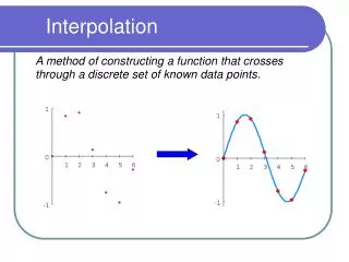
Interpolation A method of constructing a function that crosses through a discrete set of known data points. .
Spline Interpolation • Linear, Quadratic, Cubic • Preferred over other polynomial interpolation • More efficient • High-degree polynomials are very computationally expensive • Smaller error • Interpolant is smoother
Spline Interpolation Definition • Given n+1 distinct knotsxi such that: with n+1 knot values yi find a spline function with each Si(x) a polynomial of degree at most n.
Linear Spline Interpolation • Simplest form of spline interpolation • Points connected by lines Each Si is a linear function constructed as: Must be continuous at each data point: Continuity:
Quadratic Spline Interpolation • The quadratic spline can be constructed as: The coefficients can be found by choosing a z0 and then using the recurrence relation:
Quadratic Splines 2 • Quadratic splines are rarely used for interpolation for practical purposes • Ideally quadratic splines are only used to understand cubic splines
Quadratic Spline Graph t=a:2:b;
Quadratic Spline Graph t=a:0.5:b;
x t0 t1 … tn y y0 y1 … yn Natural Cubic Spline Interpolation • The domain of S is an interval [a,b]. • S, S’, S’’ are all continuous functions on [a,b]. • There are points ti (the knots of S) such that a = t0 < t1 < .. tn = b and such that S is a polynomial of degree at most k on each subinterval [ti, ti+1]. SPLINE OF DEGREE k = 3 ti are knots
Natural Cubic Spline Interpolation Si(x) is a cubic polynomial that will be used on the subinterval [ xi, xi+1 ].
Natural Cubic Spline Interpolation • Si(x) = aix3 + bix2 + cix + di • 4 Coefficients with n subintervals = 4n equations • There are 4n-2 conditions • Interpolation conditions • Continuity conditions • Natural Conditions • S’’(x0) = 0 • S’’(xn) = 0
Natural Cubic Spline Interpolation • Algorithm • Define Zi = S’’(ti) • On each [ti, ti+1] S’’ is a linear polynomial with Si’’(ti) = zi, Si’’(ti+1) = z+1 • Then • Where hi = ti+1 – ti • Integrating twice yields:
Natural Cubic Spline Interpolation • Where hi = xi+1 - xi • S’i-1(ti) = S’i(ti) • Continuity • Solve this by deriving the above equation
Natural Cubic Spline Interpolation • Algorithm: • Input: ti, yi • hi = ti+1 – ti • a • ui = 2(hi-1 + hi) • vi = 6(bi – bi-1) • Solve Az = b
Bezier Spline Interpolation • A similar but different problem: Controlling the shape of curves. Problem: given some (control) points, produce and modify the shape of a curve passing through the first and last point. http://www.ibiblio.org/e-notes/Splines/Bezier.htm
Bezier Spline Interpolation Practical Application
Bezier Spline Interpolation Idea: Build functions that are combinations of some basic and simpler functions. Basic functions: B-splines Bernstein polynomials
Bernstein Polynomials • Definition 5.5: Bernstein polynomials of degree N are defined by: • For v = 0, 1, 2, …, N, where N over v = N! / v! (N – v)! • In general there are N+1 Bernstein Polynomials of degree N. For example, the Bernstein Polynomials of degrees 1, 2, and 3 are: • 1. B0,1(t) = 1-t, B1,1(t) = t; • 2. B0,2(t) = (1-t)2, B1,2(t) = 2t(1-t), B2,2(t) = t2; • 3. B0,3(t) = (1-t)3, B1,3(t) = 3t(1-t)2, B2,3(t)=3t2(1-t), B3,3(t) = t3;
Bernstein Polynomials • Given a set of control points {Pi}Ni=0, where Pi = (xi, yi), Definition 5.6: A Bezier curve of degree N is: P(t) = Ni=0 PiBi,N(t), • Where Bi,N(t), for I = 0, 1, …, N, are the Bernstein polynomials of degree N. • P(t) is the Bezier curve • Since Pi = (xi, yi) • x(t) = Ni=0xiBi,N(t) and y(t) = Ni=0yiBi,N(t) • Easy to modify curve if points are added.
Bernstein Polynomials Example • Find the Bezier curve which has the control points (2,2), (1,1.5), (3.5,0), (4,1). Substituting the x- and y-coordinates of the control points and N=3 into the x(t) and y(t) formulas on the previous slide yields x(t) = 2B0,3(t) + 1B1,3(t) + 3.5B2,3(t) + 4B3,3(t) y(t) = 2B0,3(t) + 1.5B1,3(t) + 0B2,3(t) + 1B3,3(t)