Introduction to Computational Chemistry
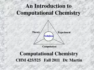
Introduction to Computational Chemistry. NSF Computational Nanotechnology and Molecular Engineering Pan-American Advanced Studies Institutes (PASI) Workshop January 5-16, 2004. California Institute of Technology, Pasadena, CA. Andrew S. Ichimura. For the Beginner….

Introduction to Computational Chemistry
E N D
Presentation Transcript
Introduction to Computational Chemistry NSF Computational Nanotechnology and Molecular Engineering Pan-American Advanced Studies Institutes (PASI) Workshop January 5-16, 2004 California Institute of Technology, Pasadena, CA Andrew S. Ichimura
For the Beginner… There are three main problems: 1. Deciphering the language. 2. Technical implementation. 3. Quality assessment.
Focus on… Calculating molecular structures and relative energies. • Hartree-Fock (Self-Consistent Field) • Electron Correlation • Basis sets and performance
Molecular properties Transition States Reaction coords. Ab initio electronic structure theory Hartree-Fock (HF) Electron Correlation (MP2, CI, CC, etc.) Spectroscopic observables Geometry prediction Prodding Experimentalists Benchmarks for parameterization Goal: Insight into chemical phenomena.
Setting up the problem… What is a molecule? A molecule is “composed” of atoms, or, more generally as a collection of charged particles, positive nuclei and negative electrons. The interaction between charged particles is described by; Coulomb Potential Coulomb interaction between these charged particles is the only important physical force necessary to describe chemical phenomena.
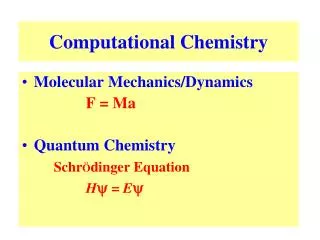
But, electrons and nuclei are in constant motion… In Classical Mechanics, the dynamics of a system (i.e. how the system evolves in time) is described by Newton’s 2nd Law: F = force a = acceleration r = position vector m = particle mass In Quantum Mechanics, particle behavior is described in terms of a wavefunction, Y. Time-dependent Schrödinger Equation Hamiltonian Operator
Time-Independent Schrödinger Equation If H is time-independent, the time-dependence of Y may be separated out as a simple phase factor. Time-Independent Schrödinger Equation Describes the particle-wave duality of electrons.
Hamiltonian for a system with N-particles Sum of kinetic (T) and potential (V) energy Kinetic energy Laplacian operator Potential energy When these expressions are used in the time-independent Schrodinger Equation, the dynamics of all electrons and nuclei in a molecule or atom are taken into account.
Born-Oppenheimer Approximation • So far, the Hamiltonian contains the following terms: • Since nuclei are much heavier than electrons, their velocities are much smaller. To a good approximation, the Schrödinger equation can be separated into two parts: • One part describes the electronic wavefunction for a fixed nuclear geometry. • The second describes the nuclear wavefunction, where the electronic energy plays the role of a potential energy.
Born-Oppenheimer Approx. cont. • In other words, the kinetic energy of the nuclei can be treated separately. This is the Born-Oppenheimer approximation. As a result, the electronic wavefunction depends only on the positions of the nuclei. • Physically, this implies that the nuclei move on a potential energy surface (PES), which are solutions to the electronic Schrödinger equation. Under the BO approx., the PES is independent of the nuclear masses; that is, it is the same for isotopic molecules. • Solution of the nuclear wavefunction leads to physically meaningful quantities such as molecular vibrations and rotations. H. + H. E 0 H H
Limitations of the Born-Oppenheimer approximation • The total wavefunction is limited to one electronic surface, i.e. a particular electronic state. • The BO approx. is usually very good, but breaks down when two (or more) electronic states are close in energy at particular nuclear geometries. In such situations, a “ non-adiabatic” wavefunction - a product of nuclear and electronic wavefunctions - must be used. • In writing the Hamiltonian as a sum of electron kinetic and potential energy terms, relativistic effects have been ignored. These are normally negligible for lighter elements (Z<36), but not for the 4th period or higher. • By neglecting relativistic effects, electron spin must be introduced in an adhoc fashion. Spin-dependent terms, e.g., spin-orbit or spin-spin coupling may be calculated as corrections after the electronic Schrödinger equation has been solved. The electronic Hamiltonian becomes, B.O. approx.; fixed nuclear coord.
Self-consistent Field (SCF) Theory GOAL: Solve the electronic Schrödinger equation, HeY=EY. PROBLEM: Exact solutions can only be found for one-electron systems, e.g., H2+. SOLUTION: Use the variational principle to generate approximate solutions. Variational principle - If an approximate wavefunction is used in HeY=EY, then the energy must be greater than or equal to the exact energy. The equality holds when Y is the exact wavefunction. In practice: Generate the “best” trial function that has a number of adjustable parameters. The energy is minimized as a function of these parameters.
SCF cont. The energy is calculated as an expectation value of the Hamiltonian operator: Introduce “bra-ket” notation, complex conjugate , left bra ket right Combined bracket denotes integration over all coordinates. If the wavefunctions are orthogonal and normalized (orthonormal), (Kroenecker delta) Then,
SCF cont. Since electrons are fermions, S=1/2,the total electronic wavefunction must be antisymmetric (change sign) with respect to the interchange of any two electron coordinates. (Pauli principle - no two electrons can have the same set of quantum numbers.) Antisymmetric wavefunctions can be written as Slater determinants. Consider a two electron system, e.g. He or H2. A suitable antisymmetric wavefunction to describe the ground state is: (He: f1 =f2 = 1s) (H2: f1 = f2 = fbonding MO) Each electron resides in a spin-orbital, a product of spatial and spin functions. Interchange the coordinates of the two electrons,
SCF cont. A more general way to represent antisymmetric electronic wavefunctions is in the form of a determinant. For the two-electron case, For an N-electron N-spinorbital wavefunction, A Slater Determinant (SD) satisfies the antisymmetry requirement. Columns are one-electron wavefunctions, molecular orbitals. Rows contain the electron coordinates. One more approximation: The trial wavefunction will consist of a single SD. Now the variational principle is used to derive the Hartree-Fock equations...
Hartree-Fock Equations (1) Reformulate the Slater Determinant as, (2) Depends on two electrons One electron terms
One-electron operator - describes electron i, moving in the field of the nuclei. Two-electron operator - interelectron repulsion. Hamiltonian (3) Calculation of the energy. Expectation value over Slater Determinant Examine specific integrals: Nuclear repulsion does not depend on electron coordinates.
For coordinate 1, The one-electron operator acts only on electron 1 and yields an energy, h1, that depends only on the kinetic energy and attraction to all nuclei. Coulomb integral, J12: represents the classical repulsion between two charge distributions f12(1) and f22(2). Exchange integral, K12: no classical analogue. Responsible for chemical bonds.
The expression for the energy can now be written as: Sum of one-electron, Coulomb, and exchange integrals, and Vnn. To apply the variational principle, the Coulomb and Exchange integrals are written as operators, The objective now is to find the best orbitals (fi, MOs) that minimize the energy (or at least remain stationary with respect to further changes in fi), while maintaining orthonormality of fi.
Employ the method of Langrange Multipliers: Function to optimize. Rewrite in terms of another function. Define Lagrange function. Constrained optimization of L. • In terms of molecular orbitals, the Langrange function is: Change in L with respect to small changes in fi should be zero. • Change in the energy with respect changes in fi.
Define the Fock Operator, Fi Effective one-electron operator, associated with the variation in the energy. Change in energy in terms of the Fock operator. According to the variational principle, the best orbitals, fi, will make dL=0. After some algebra, the final expression becomes: Hartree-Fock Equations
After a unitary transformation, lij0 and liiei. HF equations in terms of Canonical MOs and diagonal Lagrange multipliers. Lagrange multipliers can be interpreted as MO energies. Note: The HF equations cast in this way, form a set of pseudo-eigenvalue equations. A specific Fock orbital can only be determined once all the other occupied orbitals are known. The HF equations are solved iteratively. Guess, calculate the energy, improve the guess, recalculate, etc. A set of orbitals that is a solution to the HF equations are called Self-consistent Field (SCF) orbitals. The Canonical MOs are a convenient set of functions to use in the variational procedure, but they are not unique from the standpoint of calculating the energy.
Koopman’s Theorem The ionization energy is well approximated by the orbital energy, ei. * Calculated according to Koopman’s theorem.
Basis Set Approximation • For atoms and diatomic molecules, numerical HF methods are available. • In most molecular calculations, the unknown MOs are expressed in terms of a known set of functions - a basis set. Two criteria for selecting basis functions. I) They should be physically meaningful. ii) computation of the integrals should be tractable. • It is common practice to use a linear expansion of Gaussian functions in the MO basis because they are easy to handle computationally. • Each MO is expanded in a set of basis functions centered at the nuclei and are commonly called Atomic Orbitals. (Molecular orbital = Linear Combination of Atomic Orbitals - LCAO).
MO Expansion LCAO - MO representation Coefficients are variational parameters HF equations in the AO basis Matrix representation of HF eqns. Roothaan-Hall equations (closed shell) Fab - element of the Fock matrix Sab - overlap of two AOs • Roothaan-Hall equations generate M molecular orbitals from M basis functions. • N-occupied MOs • M-N virtual or unoccupied MOs (no physical interpretation)
Total Energy in MO basis Total Energy in AO basis One-electron integrals, M2 Two-electron integrals, M4 Computed at the start; do not change Products of AO coeff form Density Matrix, D
General SCF Procedure Obtain initial guess for coeff., cai,form the initial Dgd Two-electron integrals Form the Fock matrix Iterate Diagonalize the Fock Matrix Form new Density Matrix
Computational Effort • Formally, the SCF procedure scales as M4 (the number of basis functions to the 4th power). Accuracy • As the number of functions increases, the accuracy of the Molecular Orbitals improves. • As M, the complete basis set limit is reached Hartree-Fock limit. • Result: The best single determinant wavefunction that can be obtained. (This is not the exact solution to the Schrodinger equation.) Practical Limitation • In practice, a finite basis set is used; the HF limit is never reached. • The term “Hartree-Fock” is often used to describe SCF calculations with incomplete basis sets.
Restricted and Unrestricted Hartree-Fock Restricted Hartree-Fock (RHF) For even electron, closed-shell singlet states, electrons in a given MO with a and b spin are constrained to have the same spatial dependence. Restricted Open-shell Hartree-Fock (ROHF) The spatial part of the doubly occupied orbitals are restricted to be the same. Unrestricted Hartree-fock (UHF) a and b spinorbitals have different spatial parts. a b 5 4 Spinorbitals fis(n) 3 Energy 2 1 RHF Singlet ROHF Doublet UHF Doublet
Comparison of RHF and UHF • R(O)HF • a and b spins have same spatial part • Wavefunction, F, is an eigenfunction of S2 operator. • For open-shell systems, the unpaired electron (a) interacts differently with a and b spins. The optimum spatial orbitals are different. Restricted formalism is not suitable for spin dependent properties. • Starting point for more advanced calculations that include electron correlation. • UHF • a and b spins have different spatial parts • Wavefunction is not an eigenfunction of S2. F may be contaminated with states of higher multiplicity (2S+1). • EUHF ≤ ER(O)HF • Yields qualitatively correct spin densities. • Starting point for more advanced calculations that include electron correlation.
Ab Initio (latin, “from the beginning”) Quantum Chemistry Summary of approximations • Born-Oppenheimer Approx. • Non-relativistic Hamiltonian • Use of trial functions, MOs, in the variational procedure • Single Slater determinant • Basis set, LCAO-MO approx. • RHF, ROHF, UHF Consequence of using a single Slater determinant and the Self-consistent Field equations: Electron-electron repulsion is included as an average effect. The electron repulsion felt by one electron is an average potential field of all the others, assuming that their spatial distribution is represented by orbitals. This is sometimes referred to as the Mean Field Approximation. Electron correlation has been neglected!!!