Introduction to Computational Chemistry
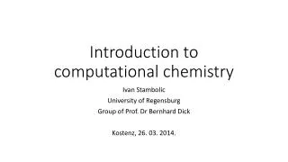
Introduction to Computational Chemistry. Shubin Liu, Ph.D. Research Computing Center University of North Carolina at Chapel Hill. Outline. Introduction Methods in Computational Chemistry Ab Initio Semi-Empirical Density Functional Theory New Developments (QM/MM) Hands-on Exercises.

Introduction to Computational Chemistry
E N D
Presentation Transcript
Introduction to Computational Chemistry Shubin Liu, Ph.D. Research Computing Center University of North Carolina at Chapel Hill
Outline • Introduction • Methods in Computational Chemistry • Ab Initio • Semi-Empirical • Density Functional Theory • New Developments(QM/MM) • Hands-on Exercises The PDF format of this presentation is available here: http://www.unc.edu/~shubin/Courses/Comp_Chem.pdf
About Us ITS – Information Technology Services http://its.unc.edu http://help.unc.edu Physical locations: 401 West Franklin St. 211 Manning Drive 10 Divisions/Departments Information SecurityIT Infrastructure and Operations Research Computing CenterTeaching and Learning User Support and EngagementOffice of the CIO Communication TechnologiesCommunications Enterprise ApplicationsFinance and Administration
Research Computing Where and who are we and what do we do? ITS Manning: 211 Manning Drive Website http://its.unc.edu/research-computing.html Groups Infrastructure -- Hardware User Support -- Software Engagement -- Collaboration
About Myself Ph.D. from Chemistry, UNC-CH Currently Senior Computational Scientist @ Research Computing Center, UNC-CH Responsibilities: Support Computational Chemistry/Physics/Material Science software Support Programming (FORTRAN/C/C++) tools, code porting, parallel computing, etc. Offer short courses on scientific computing and computational chemistry Conduct research and engagement projects in Computational Chemistry Development of DFT theory and concept tools Applications in biological and material science systems
About You Name, department, research interest? Any experience before with high performance computing? Any experience before with computational chemistry research? Do you have any real problem to solve with computational chemistry approaches?
Think BIG!!! • What is not chemistry? • From microscopic world, to nanotechnology, to daily life, to environmental problems • From life science, to human disease, to drug design • Only our mind limits its boundary • What cannot computational chemistry deal with? • From small molecules, to DNA/proteins, 3D crystals and surfaces • From species in vacuum, to those in solvent at room temperature, and to those under extreme conditions (high T/p) • From structure, to properties, to spectra (UV, IR/Raman, NMR, VCD), to dynamics, to reactivity • All experiments done in labs can be done in silico • Limited only by (super)computers not big/fast enough!
Central Theme of Computational Chemistry STRUCTURE DYNAMICS REACTIVITY CENTRAL DOGMA OF MOLECULAR BIOLOGY SEQUENCE STRUCTURE DYNAMICS FUNCTION EVALUTION
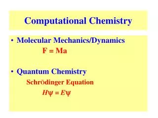
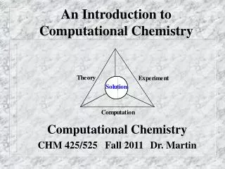
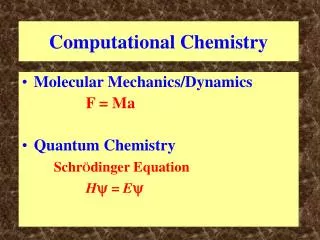
What is Computational Chemistry? Application of computational methods and algorithms in chemistry • Quantum Mechanical i.e., via Schrödinger Equation also called Quantum Chemistry • Molecular Mechanical i.e., via Newton’s law F=ma also Molecular Dynamics • Empirical/Statistical e.g., QSAR, etc., widely used in clinical and medicinal chemistry Focus Today
How Big Systems Can We Deal with? Assuming typical computing setup (number of CPUs, memory, disk space, etc.) • Ab initio method: ~100 atoms • DFT method: ~1000 atoms • Semi-empirical method: ~10,000 atoms • MM/MD: ~100,000 atoms
Equation to Solve in ab initio Theory Known exactly: 3N spatial variables (N # of electrons) To be approximated: 1. variationally 2. perturbationally
kinetic energy of the electrons kinetic energy of the nuclei electrostatic interaction between the electrons and the nuclei electrostatic interaction between the electrons electrostatic interaction between the nuclei Hamiltonian for a Molecule
Ab Initio Methods • Accurate treatment of the electronic distribution using the full Schrödinger equation • Can be systematically improved to obtain chemical accuracy • Does not need to be parameterized or calibrated with respect to experiment • Can describe structure, properties, energetics and reactivity • What does “ab intio” mean? • Start from beginning, with first principle • Who invented the word of the “ab initio” method? • Bob Parr of UNC-CH in 1950s; See Int. J. Quantum Chem.37(4), 327(1990) for details.
Three Approximations • Born-Oppenheimer approximation • Electrons act separately of nuclei, electron and nuclear coordinates are independent of each other, and thus simplifying the Schrödinger equation • Independent particle approximation • Electrons experience the ‘field’ of all other electrons as a group, not individually • Give birth to the concept of “orbital”, e.g., AO, MO, etc. • LCAO-MO approximation • Molecular orbitals (MO) can be constructed as linear combinations of atom orbitals, to form Slater determinants
Born-Oppenheimer Approximation • the nuclei are much heavier than the electrons and move more slowly than the electrons • freeze the nuclear positions (nuclear kinetic energy is zero in the electronic Hamiltonian) • calculate the electronic wave function and energy • E depends on the nuclear positions through the nuclear-electron attraction and nuclear-nuclear repulsion terms • E = 0 corresponds to all particles at infinite separation
Approximate Wavefunctions • Construction of one-electron functions (molecular orbitals, MO’s) as linear combinations of one-electron atomic basis functions (AOs) MO-LCAO approach. • Construction of N-electron wavefunction as linear combination of anti-symmetrized products of MOs (these anti-symmetrized products are denoted as Slater-determinants).
The Two Extreme Cases • One determinant: The Hartree–Fock method. • All possible determinants: The full CI method. There are N MOs and each MO is a linear combination of N AOs. Thus, there are nN coefficients ukl, which are determined by making stationary the functional: The ij are Lagrangian multipliers.
The Full CI Method • The full configuration interaction (full CI) method expands the wavefunction in terms of all possible Slater determinants: • There are possible ways to choose n molecular orbitals from a set of 2N AO basis functions. • The number of determinants gets easily much too large. For example: Davidson’s method can be used to find one or a few eigenvalues of a matrix of rank 109.
The Hartree–Fock Method Hartree–Fock equations
The Hartree–Fock Method Overlap integral Density Matrix
Self-Consistent-Field (SCF) • Choose start coefficients for MO’s • Construct Fock Matrix with coefficients • Solve Hartree-Fock-Roothaan equations • Repeat 2 and 3 until ingoing and outgoing coefficients are the same
Ab Initio Methods Semi-empirical methods (MNDO, AM1, PM3, etc.) Hartree-Fock (HF-SCF) excitation hierarchy (CIS,CISD,CISDT,...) (CCS, CCSD, CCSDT,...) perturbational hierarchy (MP2, MP3, MP4, …) excitation hierarchy (MR-CISD) perturbational hierarchy (CASPT2, CASPT3) Multiconfigurational HF (MCSCF, CASSCF) Full CI
Size vs Accuracy Full CI 0.1 Coupled-cluster, Multireference Nonlocal density functional, Perturbation theory 1 Accuracy (kcal/mol) Local density functional, Hartree-Fock 10 Semiempirical Methods 1 10 100 1000 Number of atoms
AN EXAMPLE Equilibrium structure of (H2O)2W.K., J.G.C.M. van Duijneveldt-van de Rijdt, and F.B. van Duijneveldt, Phys. Chem. Chem. Phys.2, 2227 (2000). 95.7 pm 95.8 pm ROO,e= 291.2 pm symmetry: Cs 96.4 pm Experimental [J.A. Odutola and T.R. Dyke, J. Chem. Phys 72, 5062 (1980)]: ROO2 ½ = 297.6 ± 0.4 pm SAPT-5s potential [E.M. Mas et al., J. Chem. Phys.113, 6687 (2000)]: ROO2 ½ – ROO,e= 6.3 pm ROO,e(exptl.) = 291.3 pm
Experimental and Computed Enthalpy Changes He in kJ/mol Gaussian-2 (G2) method of Pople and co-workers is a combination of MP2 and QCISD(T)
LCAO Basis Functions • ’s, which are atomic orbitals, are called basis functions • usually centered on atoms • can be more general and more flexible than atomic orbital functions • larger number of well chosen basis functions yields more accurate approximations to the molecular orbitals
Slaters (STO) Gaussians (GTO) Angular part * Better behaved than Gaussians 2-electron integrals hard 2-electron integrals simpler Wrong behavior at nucleus Decrease too fast with r Basis Functions
Minimal STO-nG Split Valence: 3-21G,4-31G, 6-31G Contracted Gaussian Basis Set • Each atom optimized STO is fit with n GTO’s • Minimum number of AO’s needed • Contracted GTO’s optimized per atom • Doubling of the number of valence AO’s
Polarization / Diffuse Functions • Polarization: Add AO with higher angular momentum (L) to give more flexibility Example: 3-21G*, 6-31G*, 6-31G**, etc. • Diffusion: Add AO with very small exponents for systems with very diffuse electron densities such as anions or excited states Example: 6-31+G*, 6-311++G**
Correlation-Consistent Basis Functions • a family of basis sets of increasing size • can be used to extrapolate to the basis set limit • cc-pVDZ – DZ with d’s on heavy atoms, p’s on H • cc-pVTZ – triple split valence, with 2 sets of d’s and one set of f’s on heavy atoms, 2 sets of p’s and 1 set of d’s on hydrogen • cc-pVQZ, cc-pV5Z, cc-pV6Z • can also be augmented with diffuse functions (aug-cc-pVXZ)
Pseudopotentials, Effective Core Potentials • core orbitals do not change much during chemical interactions • valence orbitals feel the electrostatic potential of the nuclei and of the core electrons • can construct a pseudopotential to replace the electrostatic potential of the nuclei and of the core electrons • reduces the size of the basis set needed to represent the atom (but introduces additional approximations) • for heavy elements, pseudopotentials can also include of relativistic effects that otherwise would be costly to treat
Correlation Energy • HF does not include correlations anti-parallel electrons • Eexact – EHF = Ecorrelation • Post HF Methods: • Configuration Interaction (CI, MCSCF, CCSD) • Møller-Plesset Perturbation series (MP2, MP4) • Density Functional Theory (DFT)
Configuration-Interaction (CI) • In Hartree-Fock theory, the n-electron wavefunction is approximated by one single Slater-determinant, denoted as: • This determinant is built from n orthonormal spin-orbitals. The spin-orbitals that form are said to be occupied. The other orthonormal spin-orbitals that follow from the Hartree-Fock calculation in a given one-electron basis set of atomic orbitals (AOs) are known as virtual orbitals. For simplicity, we assume that all spin-orbitals are real. • In electron-correlation or post-Hartree-Fock methods, the wavefunction is expanded in a many-electron basis set that consists of many determinants. Sometimes, we only use a few determinants, and sometimes, we use millions of them: In this notation, is a Slater- determinant that is obtained by replacing a certain number of occupied orbitals by virtual ones. • Three questions: 1. Which determinants should we include? 2. How do we determine the expansion coefficients? 3. How do we evaluate the energy (or other properties)?
Truncated configuration interaction: CIS, CISD, CISDT, etc. • We start with a reference wavefunction, for example the Hartree-Fock determinant. • We then select determinants for the wavefunction expansion by substituting orbitals of the reference determinant by orbitals that are not occupied in the reference state (virtual orbitals). • Singles (S) indicate that 1 orbital is replaced, doubles (D) indicate 2 replacements, triples (T) indicate 3 replacements, etc., leading to CIS, CISD, CISDT, etc.
Truncated Configuration Interaction Number of linear variational parameters in truncated CI for n = 10 and 2N = 40.
Multi-Configuration Self-Consistent Field (MCSCF) • The MCSCF wavefunctions consists of a few selected determinants or CSFs. In the MCSCF method, not only the linear weights of the determinants are variationally optimized, but also the orbital coefficients. • One important selection is governed by the full CI space spanned by a number of prescribed active orbitals (complete active space, CAS). This is the CASSCF method. The CASSCF wavefunction contains all determinants that can be constructed from a given set of orbitals with the constraint that some specified pairs of - and -spin-orbitals must occur in all determinants (these are the inactive doubly occupied spatial orbitals). • Multireference CI wavefunctions are obtained by applying the excitation operators to the individual CSFs or determinants of the MCSCF (or CASSCF) reference wave function. Internally-contracted MRCI:
Coupled-Cluster Theory • System of equations is solved iteratively (the convergence is accelerated by utilizing Pulay’s method, “direct inversion in the iterative subspace”, DIIS). • CCSDT model is very expensive in terms of computer resources. Approximations are introduced for the triples: CCSD(T), CCSD[T], CCSD-T. • Brueckner coupled-cluster (e.g., BCCD) methods use Brueckner orbitals that are optimized such that singles don’t contribute. • By omitting some of the CCSD terms, the quadratic CI method (e.g., QCISD) is obtained.
Møller-Plesset Perturbation Theory • The Hartree-Fock function is an eigenfunction of the n-electron operator . • We apply perturbation theory as usual after decomposing the Hamiltonian into two parts: • More complicated with more than one reference determinant (e.g., MR-PT, CASPT2, CASPT3, …) MP2, MP3, MP4, …etc. number denotes order to which energy is computed (2n+1 rule)
These methods are derived from the Hartee–Fock model, that is, they are MO-LCAO methods. They only consider the valence electrons. A minimal basis set is used for the valence shell. Integrals are restricted to one- and two-center integrals and subsequentlyparametrizedby adjusting the computed results to experimental data. Very efficient computational tools, which can yield fast quantitative estimates for a number of properties. Can be used for establishing trends in classes of related molecules, and for scanning a computational poblem before proceeding with high-level treatments. A not of elements, especially transition metals, have not be parametrized Semi-Empirical Methods
Semi-Empirical Methods • Number 2-electron integrals (mu|ls) is n4/8, n = number of basis functions • Treat only valence electrons explicit • Neglect large number of 2-electron integrals • Replace others by empirical parameters • Models: • Complete Neglect of Differential Overlap (CNDO) • Intermediate Neglect of Differential Overlap (INDO/MINDO) • Neglect of Diatomic Differential Overlap (NDDO/MNDO, AM1, PM3)
Approximations of 1-e integrals Umm from atomic spectra VAB value per atom pair m,uon the same atom One b parameter per element
Popular DFT • Noble prize in Chemistry, 1998 • In 1999, 3 of top 5 most cited journal articles in chemistry (1st, 2nd, & 4th) • In 2000-2004, top 3 most cited journal articles in chemistry • In 2005, 4 of top 5 most cited journal articles in chemistry • 1st, Becke’s hybrid exchange functional (1993) • 2nd, Lee-Yang-Parr correlation functional (1988) • 3rd, Becke’s exchange functional (1988) • 5th, PBE correlation functional (1996) http://www.cas.org/spotlight/bchem.html
Advantageous DFT • Computationally efficient Hartree-Fock-like computationally (~N3) , but included electron correlation effects • Theoretically rigorous Two Hohenberg-Kohn theorems guarantee an exact theory in ground state • Conceptually insightful Provides basis to understand chemical reactivity and other chemical properties
Brief History of DFT • First speculated 1920’ • Thomas-Fermi (kinetic energy) and Dirac (exchange energy) formulas • Officially born in 1964 with Hohenberg- Kohn’s original proof • GEA/GGA formulas available later 1980’ • Becoming popular later 1990’ • Pinnacled in 1998 with a chemistry Nobel prize
What could expect from DFT? • LDA, ~20 kcal/mol error in energy • GGA, ~3-5 kcal/mol error in energy • G2/G3 level, some systems, ~1kcal/mol • Good at structure, spectra, & other properties predictions • Poor in H-containing systems, TS, spin, excited states, etc.
Density Functional Theory • Hohenberg-Kohn theorems: • “Given the external potential, we know the ground-state energy of the molecule when we know the electron density ”. • The energy density functional is variational.