Introduction to Computational Chemistry

1. Introduction to Computational Chemistry Meredith J. T. Jordan m.jordan@chem.usyd.edu.au School of Chemistry, University of Sydney

2. Format Introductory lectures from me Master Classes from people who know what they are doing: Concurrent introductory structured workshops to introduce you to computational chemistry (me) Peter Gill Michelle Coote Haibo Yu Brian Yates Tim Clark

3. Overview Computational Chemistry: • What is Computational Chemistry • Overview • What kinds of problems can we solve? • What kinds of tools can we use? • Some examples

4. What is Computational Chemistry? Chemistry in the computer instead of in the laboratory Use computer calculations to predict the structures, reactivities and other properties of molecules Computational chemistry has become widely used because of • Dramatic increase in computer speed and the • Design of efficient quantum chemical algorithms The computer calculations enable us to • explain and rationalize known chemistry • explore new or unknown chemistry

5. Why do Chemistry on a Computer? • Calculations are easy to performwhereas experiments are difficult • Calculations are safe whereas many experiments are dangerous • Calculations are becoming less costly while experiments are becoming more expensive • Calculations can be performed on any chemical system, whereas experiments are relatively limited • Calculations give direct information whereas there is often uncertain in interpreting experimental observation • Calculations give fundamental information about isolated molecules without the complicating solvent effects

6. What Properties can be Calculated? • Equilibrium structures • Transition State structures • Microwave, NMR spectra • Reaction energies • Reaction barriers • Dissociation energies • Charge distributions • Reaction Rates • Reaction Free Energies • Circular Dichroism (optical, magnetic, vibrational) • Spin-orbit couplings • Full relativistic energies • Excited States (vertical) • Solvent Effects • pKa’s • Density matrix methods/geminals • Linear Scaling (ie of the methods with number of electrons/basis functions) • Local correlation methods • Accurate enzyme-substrate interactions • Crystal structures (prediction) • Melting points • Protein folding • Full reaction dynamics • Molecular dynamics • Solvent dynamics • Systematic improvements of DFT • Excited States (adiabatic)…

7. What Properties can be Calculated? In order of difficulty: Molecular Structures (+/– 1%) Reaction Enthalpies (+/– 2 kcal/mol) Vibrational Frequencies (+/– 10%) Reaction Free Energies (+/– 5 kcal/mol) Infrared Intensities (normally not too bad for fundamentals) Dipole Moments (depends…) Reaction Rates (errors vary enormously)

8. Conceptual Approach Validation Interpretation Prediction “…give us insight, not numbers” C. A. Coulson It is absolutely essential that we know how accurate our computed results are to be if they are to be of any use: we want to get the right answer for the right reason. A celebrated target accuracy is “Chemical Accuracy” ie to within 1 kcal/mol (~4 kJ/mol) in energy.

9. A Computational Research Project What do you want to know? How accurately? Why? This is your research project How accurate do you predict the answer will be? What is an appropriate method to use How long do you expect it to take? What method can you feasibly use What approximations are being made? Which are significant? Can you actually answer your questions Once you have finally answered all of these questions, you must determine what software is available, what it costs and how to use it.

10. Assessment Golden Rule: Before applying a particular level of theory to an experimentally unknown situation it is essential to apply the same level of theory to situations where experimental information is available Clearly unless the theory performs satisfactorily in cases where we know the answer, there is little point in using it to probe the unknown Conversely, if the theory does work well in known situations this lends confidence to the results obtained in the unknown case.

11. Flow Chart for a Calculation Molecule Coordinates Program Molecular Properties Interpretation • Cartesian • internal • different types for different purposes • Supplied • Graphically • by hand • many different ones: • AMBER, CHARMM, • GROMOS, Sybyl… • AMPAC, MOPAC, VAMP… • Gaussian, Gamess, MOLPRO… • human input: • choice! • Difficult • structures • energies • molecular orbitals • IR, NMR, UV

12. Overview of Methods Molecular mechanics, force fields easy to comprehend quickly programmed extremely fast no electrons: limited interpretability Semiempirical methods quantum method valence electrons only fast limited accuracy ab initio methods full quantum method only experimental fundamental constants in principle very high accuracy complete (all interactions are included) very time consuming (“expensive”) systematic improvement possible Density Functional Theory quantum method in principle “exact” faster than traditional ab initio variable accuracy no systematic improvement

13. Atomic Units

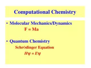
14. Starting Point: The Schrödinger Equation Foundation is the Schrödinger Equation of quantum mechanics H  = E  • Eis the energy of the system • is the molecular wavefunction.  has no simple physical meaning but 2 represents a probability distribution • His the Hamiltonian operator (a set of mathematical operations) describing the kinetic energy (T) and the potential energy (V) of the electrons and the nuclei • In principle we need to consider the electrons and nuclei in a molecule together, in practice, nuclei move much slower and we separate out electronic and nuclear motion (the Born-Oppenheimer approximation)

15. Predicting the Structure of a Molecule The Schrödinger equation allows us to calculate the energy (E) of a system as a function of geometry Predict the structure of carbon monoxide (CO) Energy R(C…O) H  = E  Re

16. Potential Energy Surfaces The Born-Oppenheimer approximation lets us consider how electronic energy changes with the nuclear geometry, giving a Molecular Potential Energy Surface multidimensional (3N-6 dimensions) describes how energy varies as the atoms in the system move, ie energy as a function of molecular displacement principally determined by what the bonding electrons (the valence electrons) are doing

17. Potential Energy Surfaces For any stationary point: • For equilibrium structures:    Local Minima

18. Equilibrium Molecular Structures Stable structures are minima energy curves upwards in all directions curvature is positive: all vibrational frequencies are real often there are lots of minima the most stable structure is the global minimum 

19. Finding Minimum Energy Structures Gradient methods Steepest descents Conjugate gradient Second derivative methods Newton-Rhapson Quasi-Newton Fletcher Powell Rational Function Optimisation 

20. Finding Minimum Energy Structures Monte Carlo Methods Metropolis sampling Simulated annealing Divide and Conquer Break the probleminto smaller, more tractable chunks http://www.cs.gmu.edu/~ashehu/?q=ProjectionGuidedExploration

21. Transition State Structures     Transition State structure • For transition state structures: 

22. Transition State Structures The maximum energy configuration along the reaction path is called the transition state energy curves downwards in one direction only There is one imaginary vibrational frequency, all other vibrational frequencies are real   

23. Finding Transition State Structures Newton-Rhapson type method Start with a good guess structure Start with accurate second derivatives Walk uphill following the least steep route   

24. Chemical Reactivity Reactions are paths on the surface the lowest energy path between reactants and products is called the intrinsic reaction path   

25. Vibrational Frequencies Indicate if the structure is a minimum (equilibrium structure - all real frequencies – or a saddle point (transition state) – one imaginary frequency – on the potential energy surface Allow us to calculate: IR and Raman spectra zero-point vibrational energy (ZPVE) useful thermochemical quantities Reaction rate coefficients Isotopic substitution effects Tunneling corrections

26. Theoretical Models “The underlying physical laws necessary for the mathematical theory of a large part of physics and the whole of chemistry are thus completely known, and the difficulty is only that the exact application of these laws leads to equations much too complicated to be soluble.” Paul Dirac 1929 (Nobel Prize 1933)