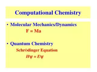
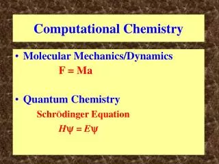
Computational Chemistry

1. Computational Chemistry An Introduction to Molecular Dynamic Simulations Shalayna Lair Molecular Mechanics, Chem 5369 University of Texas at El Paso

2. “Computational chemistry simulates chemical structures and reactions numerically, based in full or in part on the fundamental laws of physics.” Foresman and Frisch In Exploring Chemistry with Electronic Structure Methods, 1996

3. Outline • Introduction • Schrödinger's Equation • How to Conduct a Project • Type of Calculations • Computational Models • Molecular Mechanics • Semi Empirical • Ab Initio • Density Functional Theory • Basis Sets • Accuracy Comparison • Summary

4. Introduction • Computational chemistry is a branch of chemistry concerned with theoretically determining properties of molecules. • Because of the difficulty of dealing with nanosized materials, computational modeling has become an important characterization tool in nanotechnology.

5. Schrödinger’s Equation: Hψ = Eψ • The Schrödinger equation is the basis of quantum mechanics and gives a complete description of the electronic structure of a molecule. If the equation could be fully solved all information pertaining to a molecule could be determined. • Complex mathematical equation that completely describes the chemistry of a molecular system. • Not solvable for systems with many atoms. • Due to the difficulty of the equation computers are used in conjunction with simplifications and parameterizations to solve the equation. • Describes both the wave and particle behavior of electrons. • The wavefunction is described by ψ while the particle behavior is represented by E. • In systems with more than one electron, the wavefunction is dependent on the position of the atoms; this makes it important to have an accurate geometric description of a system.

6. Development of the Schrödinger equation from other fundamental laws of physics. Erwin Schrödinger, 1927 Schrödinger Cont… http://hyperphysics.phy-astr.gsu.edu/hbase/quantum/schr.html

7. “Anyone can do calculations nowadays. Anyone can also operate a scalpel. That doesn’t mean all our medical problems are solved.” Karl Irikura

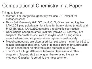
8. Conducting a Computational Project • These questions should be answered • What do you want to know? • How accurate does the prediction need to be? • How much time can be devoted to the problem? • What approximations are being made? • The answers to these questions will determine the type of calculation, model and basis set to be used. * from D. Young

9. There are three basic types of calculations. From these calculations, other information can be determined. Single-Point Energy: predict stability, reaction mechanisms Geometry Optimization: predict shape Frequency: predict spectra Atomic model of a Buckyball (C60) Types of Calculations

10. Computational Models • A model is a system of equations, or computations used to determine the energetics of a molecule • Different models use different approximations (or levels of theory) to produce results of varying levels of accuracy. • There is a trade off between accuracy and computational time. • There are two main types of models; those that use Schrödinger's equation (or simplifications of it) and those that do not.

11. Computational Models • Types of Models (Listed in order from most to least accurate) • Ab initio • uses Schrödinger's equation, but with approximations • Semi Empirical • uses experimental parameters and extensive simplifications of Schrödinger's equation • Molecular Mechanics • does not use Schrödinger's equation Simulated (12,0) zigzag carbon nanotube

12. Ab Initio • Ab initio translated from Latin means “from first principles.” This refers to the fact that no experimental data is used and computations are based on quantum mechanics. • Different Levels of Ab Initio Calculations • Hartree-Fock (HF) • The simplest ab initio calculation • The major disadvantage of HF calculations is that electron correlation is not taken into consideration. • The Møller-Plesset Perturbation Theory (MP) • Density Functional Theory (DFT) • Configuration Interaction (CI) Take into consideration electron correlation

13. Ab Initio • Approximations used in some ab initio calculations • Central field approximation: integrates the electron-electron repulsion term, giving an average effect instead of an explicit energy • Linear combination of atomic orbitals (LCAO): is used to describe the wave function and these functions are then combined into a determinant. This allows the equation to show that an electron was put in an orbital, but the electron cannot be specified.

14. Density Functional Theory • Considered an ab initio method, but different from other ab initio methods because the wavefunction is not used to describe a molecule, instead the electron density is used. • Three types of DFT calculations exist: • local density approximation (LDA) – fastest method, gives less accurate geometry, but provides good band structures • gradient corrected - gives more accurate geometries • hybrids (which are a combination of DFT and HF methods) - give more accurate geometries

15. DFT: -6139.46 HF: -6132.89 % Difference: 0.11% (units: a.u.) DFT • These types of calculations are fast becoming the most relied upon calculations for nanotube and fullerene systems. • DFT methods take less computational time than HF calculations and are considered more accurate • This (15,0) short zigzag carbon nanotube was simulated with two different models: Hartree-Fock and DFT. The differences in energetics are shown in the table.

16. Semi Empirical • Semi empirical methods use experimental data to parameterize equations • Like the ab initio methods, a Hamiltonian and wave function are used • much of the equation is approximated or eliminated • Less accurate than ab initio methods but also much faster • The equations are parameterized to reproduce specific results, usually the geometry and heat of formation, but these methods can be used to find other data.

17. Molecular Mechanics • Simplest type of calculation • Used when systems are very large and approaches that are more accurate become to costly (in time and memory) • Does not use any quantum mechanics instead uses parameters derived from experimental or ab initio data • Uses information like bond stretching, bond bending, torsions, electrostatic interactions, van der Waals forces and hydrogen bonding to predict the energetics of a system • The energy associated with a certain type of bond is applied throughout the molecule. This leads to a great simplification of the equation • It should be clarified that the energies obtained from molecular mechanics do not have any physical meaning, but instead describe the difference between varying conformations (type of isomer). Molecular mechanics can supply results in heat of formation if the zero of energy is taken into account.

18. Basis Sets • In chemistry a basis set is a group of mathematical functions used to describe the shape of the orbitals in a molecule, each basis set is a different group of constants used in the wavefunction of the Schrödinger equation. • The accuracy of a calculation is dependent on both the model and the type of basis set applied to it. • Once again there is a trade off between accuracy and time. Larger basis sets will describe the orbitals more accurately but take longer to solve. • General expression for a basis function = N * e(- * r) • where: N is the normalization constant,  is the orbital exponent, and r is the radius of the orbital in angstroms.

19. Examples of Basis Sets • STO-3G basis set - simplest basis set, uses the minimal number of functions to describe each atom in the molecule • for nanotube systems this means hydrogen is described by one function (for the 1s orbital), while carbon is described by five functions (1s, 2s, 2px, 2py and 2pz). • Split valence basis sets use two functions to describe different sizes of the same orbitals. • For example with a split valence basis set H would be described by two functions while C would be described by 10 functions. • 6-31G or 6-311G (which uses three functions for each orbital, a triple split valence set). • Polarized basis sets - improve accuracy by allowing the shape of orbitals to change by adding orbitals beyond that which is necessary for an atom • 6-31G(d) (also known as the 6-31G*) - adds a d function to carbon atoms

20. “The underlying physical laws necessary for the mathematical theory of a large part of physics and the whole of chemistry are thus completely known, and the difficulty is only that the exact application of these laws leads to equations much too complicated to be soluble.” P.A.M. Dirac, 1929

21. Accuracy Comparison Table 1. Comparison of the accuracy of different models and basis sets to experimental data. *mean absolute deviation

22. Summary • Schrödinger's equation is the basis of computational chemistry, if it could be solved all electronic information for a molecule would be known. • Since Schrödinger's equation cannot be completely solved for molecules with more than a few atoms, computers are used to solve approximations of the equation. • The level of accuracy and computational time of a simulation is dependent on the model and basis set used.

23. References • Chem Viz at http://www.shodor.org/chemviz/basis/students/introduction.html • D. YOUNG, in “Computational Chemistry, A Practical Guide for Applying Techniques to Real World Problems” (Wiley-Interscience, New York, 2001). • J. SIMMONS, in An Introduction to Theoretical Chemistry” (Cambridge Press, Cambridge, 2003). • J. B. FORESMAN AND Æ. FRISCH, in “Exploring Chemistry with Electronic Structure Methods, 2nd Edition” (Gaussian, Inc., Pittsburgh, PA, 1996).