Lecture 8 - Turbulence Applied Computational Fluid Dynamics
520 likes | 1.56k Vues
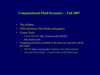
Lecture 8 - Turbulence Applied Computational Fluid Dynamics. Instructor: André Bakker. © André Bakker (2002-2005) © Fluent Inc. (2002). Turbulence. What is turbulence? Effect of turbulence on Navier-Stokes equations. Reynolds averaging. Reynolds stresses. Instability.

Lecture 8 - Turbulence Applied Computational Fluid Dynamics
E N D
Presentation Transcript
Lecture 8 - TurbulenceApplied Computational Fluid Dynamics Instructor: André Bakker © André Bakker (2002-2005) © Fluent Inc. (2002)
Turbulence • What is turbulence? • Effect of turbulence on Navier-Stokes equations. • Reynolds averaging. • Reynolds stresses.
Instability • All flows become unstable above a certain Reynolds number. • At low Reynolds numbers flows are laminar. • For high Reynolds numbers flows are turbulent. • The transition occurs anywhere between 2000 and 1E6, depending on the flow. • For laminar flow problems, flows can be solved using the conservation equations developed previously. • For turbulent flows, the computational effort involved in solving those for all time and length scales is prohibitive. • An engineering approach to calculate time-averaged flow fields for turbulent flows will be developed.
Time What is turbulence? • Unsteady, aperiodic motion in which all three velocity components fluctuate, mixing matter, momentum, and energy. • Decompose velocity into mean and fluctuating parts: Ui(t) Ui + ui(t). • Similar fluctuations for pressure, temperature, and species concentration values.
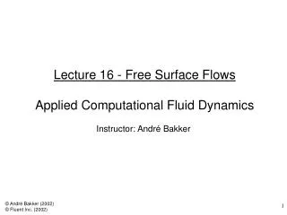
jet wake mixing layer Examples of simple turbulent flows • Some examples of simple turbulent flows are a jet entering a domain with stagnant fluid, a mixing layer, and the wake behind objects such as cylinders. • Such flows are often used as test cases to validate the ability of computational fluid dynamics software to accurately predict fluid flows.
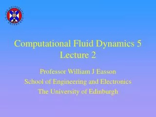
The photographs show the flow in a boundary layer. Below Recrit the flow is laminar and adjacent fluid layers slide past each other in an orderly fashion. The flow is stable. Viscous effects lead to small disturbances being dissipated. Above the transition point Recrit small disturbances in the flow start to grow. A complicated series of events takes place that eventually leads to the flow becoming fully turbulent. Transition
Transition in boundary layer flow over flat plate Turbulent spots Fully turbulent flow T-S waves
Turbulent boundary layer Top view Side view Merging of turbulent spots and transition to turbulence in a natural flat plate boundary layer.
Turbulent boundary layer Close-up view of the turbulent boundary layer.
Instability and turbulence is also seen in internal flows such as channels and ducts. The Reynolds number is constant throughout the pipe and is a function of flow rate, fluid properties and diameter. Three flow regimes are shown: Re < 2200 with laminar flow. Re = 2200 with a flow that alternates between turbulent and laminar. This is called transitional flow. Re > 2200 with fully turbulent flow. Transition in a channel flow
Small Structure Large Structure Large-scale vs. small-scale structure
As air flows over and around objects in its path, spiraling eddies, known as Von Karman vortices, may form. The vortices in this image were created when prevailing winds sweeping east across the northern Pacific Ocean encountered Alaska's Aleutian Islands Alaska's Aleutian Islands
20 km Alexander Selkirk Island in the southern Pacific Ocean
Smoke ring A smoke ring (green) impinges on a plate where it interacts with the slow moving smoke in the boundary layer (pink). The vortex ring stretches and new rings form. The size of the vortex structures decreases over time.
Simulation – species mixing Arthur Shaw and Robert Haehnel, 2004
Homogeneous, decaying, grid-generated turbulence Turbulence is generated at the grid as a result of high stresses in the immediate vicinity of the grid. The turbulence is made visible by injecting smoke into the flow at the grid. The eddies are visible because they contain the smoke. Beyond this point, there is no source of turbulence as the flow is uniform. The flow is dominated by convection and dissipation. For homogeneous decaying turbulence, the turbulent kinetic energy decreases with distance from grid as x-1 and the turbulent eddies grows in size as x1/2.
Flow transitions around a cylinder • For flow around a cylinder, the flow starts separating at Re = 5. For Re below 30, the flow is stable. Oscillations appear for higher Re. • The separation point moves upstream, increasing drag up to Re = 2000. Re = 9.6 Re = 13.1 Re = 26 Re = 10,000 Re = 30.2 Re = 2000
Turbulence: high Reynolds numbers Turbulent flows always occur at high Reynolds numbers. They are caused by the complex interaction between the viscous terms and the inertia terms in the momentum equations. Turbulent, high Reynolds number jet Laminar, low Reynolds number free stream flow
Turbulent flows are chaotic One characteristic of turbulent flows is their irregularity or randomness. A full deterministic approach is very difficult. Turbulent flows are usually described statistically. Turbulent flows are always chaotic. But not all chaotic flows are turbulent.
Turbulence: diffusivity The diffusivity of turbulence causes rapid mixing and increased rates of momentum, heat, and mass transfer. A flow that looks random but does not exhibit the spreading of velocity fluctuations through the surrounding fluid is not turbulent. If a flow is chaotic, but not diffusive, it is not turbulent.
Turbulence: dissipation Turbulent flows are dissipative. Kinetic energy gets converted into heat due to viscous shear stresses. Turbulent flows die out quickly when no energy is supplied. Random motions that have insignificant viscous losses, such as random sound waves, are not turbulent.
Turbulence: rotation and vorticity Turbulent flows are rotational; that is, they have non-zero vorticity. Mechanisms such as the stretching of three-dimensional vortices play a key role in turbulence. Vortices
What is turbulence? • Turbulent flows have the following characteristics: • One characteristic of turbulent flows is their irregularity or randomness. A full deterministic approach is very difficult. Turbulent flows are usually described statistically. Turbulent flows are always chaotic. But not all chaotic flows are turbulent. Waves in the ocean, for example, can be chaotic but are not necessarily turbulent. • The diffusivity of turbulence causes rapid mixing and increased rates of momentum, heat, and mass transfer. A flow that looks random but does not exhibit the spreading of velocity fluctuations through the surrounding fluid is not turbulent. If a flow is chaotic, but not diffusive, it is not turbulent. The trail left behind a jet plane that seems chaotic, but does not diffuse for miles is then not turbulent. • Turbulent flows always occur at high Reynolds numbers. They are caused by the complex interaction between the viscous terms and the inertia terms in the momentum equations. • Turbulent flows are rotational; that is, they have non-zero vorticity. Mechanisms such as the stretching of three-dimensional vortices play a key role in turbulence.
What is turbulence? - Continued • Turbulent flows are dissipative. Kinetic energy gets converted into heat due to viscous shear stresses. Turbulent flows die out quickly when no energy is supplied. Random motions that have insignificant viscous losses, such as random sound waves, are not turbulent. • Turbulence is a continuum phenomenon. Even the smallest eddies are significantly larger than the molecular scales. Turbulence is therefore governed by the equations of fluid mechanics. • Turbulent flows are flows. Turbulence is a feature of fluid flow, not of the fluid. When the Reynolds number is high enough, most of the dynamics of turbulence are the same whether the fluid is an actual fluid or a gas. Most of the dynamics are then independent of the properties of the fluid.
Log E Integral scale Taylor scale Kolmogorov scale Wavenumber Kolmogorov energy spectrum • Energy cascade, from largescale to small scale. • E is energy contained in eddies of wavelength l. • Length scales: • Largest eddies. Integral length scale (k3/2/e). • Length scales at which turbulence is isotropic. Taylor microscale (15nu’2/e)1/2. • Smallest eddies. Kolmogorov length scale (n3/e)1/4. These eddies have a velocity scale (n.e)1/4 and a time scale (n/e)1/2.
Vorticity and vortex stretching • Existence of eddies implies rotation or vorticity. • Vorticity concentrated along contorted vortex lines or bundles. • As end points of a vortex line move randomly further apart the vortex line increases in length but decreases in diameter. Vorticity increases because angular momentum is nearly conserved. Kinetic energy increases at rate equivalent to the work done by large-scale motion that stretches the bundle. • Viscous dissipation in the smallest eddies converts kinetic energy into thermal energy. • Vortex-stretching cascade process maintains the turbulence and dissipation is approximately equal to the rate of production of turbulent kinetic energy. • Typically energy gets transferred from the large eddies to the smaller eddies. However, sometimes smaller eddies can interact with each other and transfer energy to the (i.e. form) larger eddies, a process known as backscatter.
t3 t2 t1 t4 t5 t6 (Baldyga and Bourne, 1984) Vortex stretching
Is the flow turbulent? External flows: where along a surface L = x, D, Dh, etc. around an obstacle Other factors such as free-stream turbulence, surface conditions, and disturbances may cause earlier transition to turbulent flow. Internal flows: Natural convection: where
Turbulence modeling objective • The objective of turbulence modeling is to develop equations that will predict the time averaged velocity, pressure, and temperature fields without calculating the complete turbulent flow pattern as a function of time. • This saves us a lot of work! • Most of the time it is all we need to know. • We may also calculate other statistical properties, such as RMS values. • Important to understand: the time averaged flow pattern is a statistical property of the flow. • It is not an existing flow pattern! • It does not usually satisfy the steady Navier-Stokes equations! • The flow never actually looks that way!!
The figures show: An experimental snapshot. Streamlines for time averaged flow field. Note the difference between the time averaged and the instantaneous flow field. Effective viscosity used to predict time averaged flow field. Example: flow around a cylinder at Re=1E4 Experimental Snapshot Streamlines Effective Viscosity
Velocity decomposition • Velocity and pressure decomposition: • Turbulent kinetic energy k (per unit mass) is defined as: • Continuity equation: • Next step, time average the momentum equation. This results in the Reynolds equations.
Reynolds stresses • These equations contain an additional stress tensor. These are called the Reynolds stresses. • In turbulent flow, the Reynolds stresses are usually large compared to the viscous stresses. • The normal stresses are always non-zero because they contain squared velocity fluctuations. The shear stresses would be zero if the fluctuations were statistically independent. However, they are correlated (amongst other reasons because of continuity) and the shear stresses are therefore usually also non-zero.
Turbulent flow - continuity and scalars • Continuity: • Scalar transport equation: • Notes on density: • Here r is the mean density. • This form of the equations is suitable for flows where changes in the mean density are important, but the effect of density fluctuations on the mean flow is negligible. • For flows with Ti<5% this is up to Mach 5 and with Ti<20% this is valid up to around Mach 1.
Closure modeling • The time averaged equations now contain six additional unknowns in the momentum equations. • Additional unknowns have also been introduced in the scalar equation. • Turbulent flows are usually quite complex, and there are no simple formulae for these additional terms. • The main task of turbulence modeling is to develop computational procedures of sufficient accuracy and generality for engineers to be able to accurately predict the Reynolds stresses and the scalar transport terms. • This will then allow for the computation of the time averaged flow and scalar fields without having to calculate the actual flow fields over long time periods.