The Multiple Regression Model and its interpretation

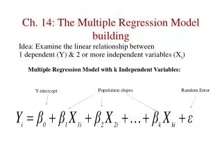
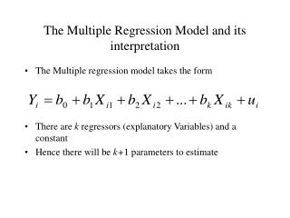
1. The Multiple Regression Model and its interpretation • The Multiple regression model takes the form • There are k regressors (explanatory Variables) and a constant • Hence there will be k+1 parameters to estimate

2. Assumption M.1 • We will keep the basic least squares assumption - We will assume that the error term is mean independent of all regressors (loosely speaking - all Xs are uncorrelated with the error term, i.e.

3. Interpretation of the coefficients • Since the error term is mean independent of the Xs (M.1) varrying the X’s does not have an impact on the error term. • Thus under Assumption M.1 the coefficients in the regression model have the following simple interpretation: • Thus each coefficient measures the impact of the corresponding X on Y keeping all other factors (Xs and u) constant.A ceteris paribus effect.

4. Example: Male wages at 33 and the Student Teacher ratio in Secondary School National Child Development Survey Data on all people born in the second week of March 1958 . regress lhw_5 strat_3 lowabil payrsed mayrsed Number of obs = 1523 F( 4, 1518) = 32.59 Prob > F = 0.0000 R-squared = 0.0761 Root MSE = .40571 ------------------------------------------------------------------------------ Log Wage rate at 33 (Men) lhw_5 | Coef. Std. Err. t P>|t| [95% Conf. Interval] -------------+---------------------------------------------------------------- Student Teacher Ratio (sec sch) strat_3 | -.0231986 .005419 -4.28 0.000 -.0338281 -.012569 Below median ability lowabil | -.1870087 .0216397 -8.64 0.000 -.2294554 -.1445619 Father’s Years of education payrsed | .012372 .0047924 2.58 0.010 .0029716 .0217723 Mother’s Years of education mayrsed| -.0058386 .0050984 -1.15 0.252 -.0158393 .0041621 _cons | 2.476687 .0952986 25.99 0.000 2.289756 2.663618 ------------------------------------------------------------------------------

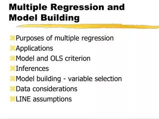
5. Least Squares in the Multiple Regression Model • We maintain the same set of assumptions as in the two variable regression model. • We modify assumption 1 to assumption M1 to take into account the existence of many regressors. • The OLS estimator is chosen to minimise the residual sum of squares exactly as before. • Thus are chosen to minimise

6. The Normal Equations • Differentiating S with respect to each coefficient in turn we obtain a set of k+1 equations constituting the first order conditions for minimising the residual sum of squares S. These equations are called the Normal Equations.

7. The Normal Equations

8. Solving the normal equations for provides the OLS estimator. • We have dealt with the special case of k=1. • From the first equation corresponding to the constant we get that • In the above the bar denotes sample mean and the hat denotes the solution to the normal equations. • This is a direct generalisation of the result for the constant term that we had in the two variable regression model. • We substitute this expression in the remaining equations and obtain

10. A solution for two regressors • With two regressors this represents a two equation system with two unknowns, i.e. • We have already solved for the constant term • The solution for is

11. This formula can also be written as • Similarly we can derive the formula for the other coefficient ( ) • Note that the formula for is now different from the formula we had in the two variable regression model. This now takes into account the presence of the other regressor(s) • The extent to which the two formulae differ depends on the covariance of and . • When this covariance is zero we are back to the formula for the one variable regression model. • This result is of significance and will be discussed in the context of omitted variable bias in a later lecture

12. Assumption M.4 • The Gauss Markov Theorem is valid for the multiple regression model. We need however to modify assumption A.4. • Define the covariance matrix of the regressors X to be • We assume that cov(X)positive definite and hence can be inverted.

13. The Gauss Markov Theorem • Theorem: Under Assumptions M.1 A.2 and A3 and M.4 the Ordinary Least Squares Estimator (OLS) is Best in the class of Linear Unbiased estimators (BLUE). • As before this means that OLS provides estimates that are least sensitive to changes in the data - given the stated assumptions.

14. The Coefficient of Determination • The is defined in exactly the same way as in the two variable regression model and measures the goodness of fit of the model. • By goodness of fit we mean the proportion of the variance of the dependent variable that is explained by the model.

15. Omitted Variable Bias • Suppose the true regression relationship has the form • Instead we decide to estimate • We will show that in general this omission will lead to a biased estimate of X1

16. Suppose we use OLS on the second equation. As we know we will obtain: • The question is : What is the expected value of the last expression on the right hand side. For an unbiased estimator this will be zero. Here we will show that it is not zero. • First note that according to the true model (i.e. the model on the top of the previous slide) we have that

17. We can substitute this into the expression for the OLS estimator to obtain • Now we can take expectations of this expression. • The last expression is zero under the assumption that u is mean independent of X [Assumption M.1]

18. The omitted variable bias expression • Thus we are left with an expression for the OLS. The last term on the right hand side is now a bias term due to the omission of a regressor. • This expression can be written more compactly as

19. The bias will be zero in two cases: • When the coefficient b2is zero. In this case the regressor X2 obviously does not belong to the regression. • When the covariance between the two regressors X1 and X2 iszero • Thus in general omitting regressors which have an impact on Y (b2 non-zero) will bias the OLS estimator of the coefficients on the included regressorsunless the omitted regressors are uncorrelated with the included ones.