The Multiple Regression Model
The Multiple Regression Model. Chapter Contents. 5.1 Introduction 5.2 Estimating the Parameters of the Multiple Regression Model 5 .3 Sampling Properties of the Least Squares Estimators 5 .4 Interval Estimation 5 .5 Hypothesis Testing 5 .6 Polynomial Equations


The Multiple Regression Model
E N D
Presentation Transcript
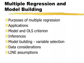
Chapter Contents • 5.1 Introduction • 5.2 Estimating the Parameters of the Multiple Regression Model • 5.3 Sampling Properties of the Least Squares Estimators • 5.4 Interval Estimation • 5.5 Hypothesis Testing • 5.6 Polynomial Equations • 5.7 Interaction Variables • 5.8 Measuring Goodness-of-fit
5.1 Introduction
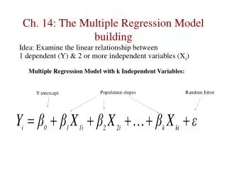
5.1 Introduction • Let’s set up an economic model in which sales revenue depends on one or more explanatory variables • We initially hypothesize that sales revenue is linearly related to price and advertising expenditure • The economic model is: Eq. 5.1
5.1 Introduction • In most economic models there are two or more explanatory variables • When we turn an economic model with more than one explanatory variable into its corresponding econometric model, we refer to it as a multiple regression model • Most of the results we developed for the simple regression model can be extended naturally to this general case 5.1.1 The Economic Model
5.1 Introduction • β2 is the change in monthly sales SALES ($1000) when the price index PRICE is increased by one unit ($1), and advertising expenditure ADVERT is held constant 5.1.1 The Economic Model
5.1 Introduction • Similarly, β3 is the change in monthly sales SALES ($1000) when the advertising expenditure is increased by one unit ($1000), and the price index PRICE is held constant 5.1.1 The Economic Model
5.1 Introduction • The econometric model is: • To allow for a difference between observable sales revenue and the expected value of sales revenue, we add a random error term, e = SALES - E(SALES) 5.1.2 The Econometric Model Eq. 5.2
5.1 Introduction FIGURE 5.1 The multiple regression plane 5.1.2 The Econometric Model
Table 5.1 Observations on Monthly Sales, Price, and Advertising in Big Andy’s Burger Barn 5.1 Introduction 5.1.2 The Econometric Model
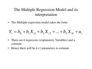
5.1 Introduction 5.1.2a The General Model • In a general multiple regression model, a dependent variable y is related to a number of explanatory variables x2, x3, …, xK through a linear equation that can be written as: Eq. 5.3
5.1 Introduction 5.1.2a The General Model • A single parameter, call it βk, measures the effect of a change in the variable xk upon the expected value of y, all other variables held constant
5.1 Introduction 5.1.2a The General Model • The parameter β1 is the intercept term. • We can think of it as being attached to a variable x1 that is always equal to 1 • That is, x1 = 1
5.1 Introduction 5.1.2a The General Model • The equation for sales revenue can be viewed as a special case of Eq. 5.3 where K = 3, y = SALES, x1 = 1, x2 = PRICE and x3 = ADVERT Eq. 5.4
5.1 Introduction • We make assumptions similar to those we made before: • E(e) = 0 • var(e) = σ2 • Errors with this property are said to be homoskedastic • cov(ei,ej) = 0 • e ~ N(0, σ2) 5.1.2b The Assumptions of the Model
5.1 Introduction • The statistical properties of y follow from those of e: • E(y) = β1 + β2x2 + β3x3 • var(y) = var(e) = σ2 • cov(yi, yj) = cov(ei, ej) = 0 • y ~ N[(β1 + β2x2 + β3x3), σ2] • This is equivalent to assuming that e ~ N(0, σ2) 5.1.2b The Assumptions of the Model
5.1 Introduction • We make two assumptions about the explanatory variables: • The explanatory variables are not random variables • We are assuming that the values of the explanatory variables are known to us prior to our observing the values of the dependent variable 5.1.2b The Assumptions of the Model
5.1 Introduction • We make two assumptions about the explanatory variables (Continued): • Any one of the explanatory variables is not an exact linear function of the others • This assumption is equivalent to assuming that no variable is redundant • If this assumption is violated – a condition called exact collinearity - the least squares procedure fails 5.1.2b The Assumptions of the Model
5.1 Introduction ASSUMPTIONS of the Multiple Regression Model 5.1.2b The Assumptions of the Model
5.2 Estimating the Parameters of the Multiple Regression Model
5.2 Estimating the Parameters of the Multiple Regression Model • We will discuss estimation in the context of the model in Eq. 5.4, which we repeat here for convenience, with i denoting the ith observation • This model is simpler than the full model, yet all the results we present carry over to the general case with only minor modifications Eq. 5.4
5.2 Estimating the Parameters of the Multiple Regression Model • Mathematically we minimize the sum of squares function S(β1, β2, β3), which is a function of the unknown parameters, given the data: 5.2.1 Least Squares Estimation Procedure Eq. 5.5
5.2 Estimating the Parameters of the Multiple Regression Model • Formulas for b1, b2, and b3, obtained by minimizing Eq. 5.5, are estimation procedures, which are called the least squares estimators of the unknown parameters • In general, since their values are not known until the data are observed and the estimates calculated, the least squares estimators are random variables 5.2.1 Least Squares Estimation Procedure
5.2 Estimating the Parameters of the Multiple Regression Model 5.2.2 Least Squares Estimates Using Hamburger Chain Data • Estimates along with their standard errors and the equation’s R2 are typically reported in equation format as: Eq. 5.6
5.2 Estimating the Parameters of the Multiple Regression Model Table 5.2 Least Squares Estimates for Sales Equation for Big Andy’s Burger Barn 5.2.2 Least Squares Estimates Using Hamburger Chain Data
5.2 Estimating the Parameters of the Multiple Regression Model 5.2.2 Least Squares Estimates Using Hamburger Chain Data • Interpretations of the results: • The negative coefficient on PRICE suggests that demand is price elastic; we estimate that, with advertising held constant, an increase in price of $1 will lead to a fall in monthly revenue of $7,908 • The coefficient on advertising is positive; we estimate that with price held constant, an increase in advertising expenditure of $1,000 will lead to an increase in sales revenue of $1,863
5.2 Estimating the Parameters of the Multiple Regression Model 5.2.2 Least Squares Estimates Using Hamburger Chain Data • Interpretations of the results (Continued): • The estimated intercept implies that if both price and advertising expenditure were zero the sales revenue would be $118,914 • Clearly, this outcome is not possible; a zero price implies zero sales revenue • In this model, as in many others, it is important to recognize that the model is an approximation to reality in the region for which we have data • Including an intercept improves this approximation even when it is not directly interpretable
5.2 Estimating the Parameters of the Multiple Regression Model 5.2.2 Least Squares Estimates Using Hamburger Chain Data • Using the model to predict sales if price is $5.50 and advertising expenditure is $1,200: • The predicted value of sales revenue for PRICE = 5.5 and ADVERT =1.2 is $77,656.
5.2 Estimating the Parameters of the Multiple Regression Model 5.2.2 Least Squares Estimates Using Hamburger Chain Data • A word of caution is in order about interpreting regression results: • The negative sign attached to price implies that reducing the price will increase sales revenue. • If taken literally, why should we not keep reducing the price to zero? • Obviously that would not keep increasing total revenue • This makes the following important point: • Estimated regression models describe the relationship between the economic variables for values similar to those found in the sample data • Extrapolating the results to extreme values is generally not a good idea • Predicting the value of the dependent variable for values of the explanatory variables far from the sample values invites disaster
5.2 Estimating the Parameters of the Multiple Regression Model 5.2.3 Estimation of the Error Variance σ2 • We need to estimate the error variance, σ2 • Recall that: • But, the squared errors are unobservable, so we develop an estimator for σ2 based on the squares of the least squares residuals:
5.2 Estimating the Parameters of the Multiple Regression Model 5.2.3 Estimation of the Error Variance σ2 • An estimator for σ2 that uses the information from and has good statistical properties is: where K is the number of β parameters being estimated in the multiple regression model. Eq. 5.7
5.2 Estimating the Parameters of the Multiple Regression Model 5.2.3 Estimation of the Error Variance σ2 • For the hamburger chain example:
5.2 Estimating the Parameters of the Multiple Regression Model 5.2.3 Estimation of the Error Variance σ2 • Note that: • Also, note that • Both quantities typically appear in the output from your computer software • Different software refer to it in different ways.
5.3 Sampling Properties of the Least Squares Estimators
5.3 Sampling Properties of the Least Squares Estimators • THE GAUSS-MARKOV THEOREM For the multiple regression model, if assumptions MR1–MR5 hold, then the least squares estimators are the best linear unbiased estimators (BLUE) of the parameters.
5.3 Sampling Properties of the Least Squares Estimators • If the errors are not normally distributed, then the least squares estimators are approximately normally distributed in large samples • What constitutes ‘‘large’’ is tricky • It depends on a number of factors specific to each application • Frequently, N – K = 50 will be large enough
5.3 Sampling Properties of the Least Squares Estimators 5.3.1 The Variances and Covariances of the Least Squares Estimators • We can show that: where Eq. 5.8 Eq. 5.9
5.3 Sampling Properties of the Least Squares Estimators 5.3.1 The Variances and Covariances of the Least Squares Estimators • We can see that: • Larger error variances 2 lead to larger variances of the least squares estimators • Larger sample sizes N imply smaller variances of the least squares estimators • More variation in an explanatory variable around its mean, leads to a smaller variance of the least squares estimator • A larger correlation between x2 and x3 leads to a larger variance of b2
5.3 Sampling Properties of the Least Squares Estimators 5.3.1 The Variances and Covariances of the Least Squares Estimators • We can arrange the variances and covariances in a matrix format:
5.3 Sampling Properties of the Least Squares Estimators 5.3.1 The Variances and Covariances of the Least Squares Estimators • Using the hamburger data: Eq. 5.10
5.3 Sampling Properties of the Least Squares Estimators 5.3.1 The Variances and Covariances of the Least Squares Estimators • Therefore, we have:
5.3 Sampling Properties of the Least Squares Estimators 5.3.1 The Variances and Covariances of the Least Squares Estimators • We are particularly interested in the standard errors:
5.3 Sampling Properties of the Least Squares Estimators Table 5.3 Covariance Matrix for Coefficient Estimates 5.3.1 The Variances and Covariances of the Least Squares Estimators
5.3 Sampling Properties of the Least Squares Estimators 5.3.2 The Distribution of the Least Squares Estimators • Consider the general for of a multiple regression model: • If we add assumption MR6, that the random errors ei have normal probability distributions, then the dependent variable yi is normally distributed:
5.3 Sampling Properties of the Least Squares Estimators 5.3.2 The Distribution of the Least Squares Estimators • Since the least squares estimators are linear functions of dependent variables, it follows that the least squares estimators are also normally distributed:
5.3 Sampling Properties of the Least Squares Estimators 5.3.2 The Distribution of the Least Squares Estimators • We can now form the standard normal variable Z: Eq. 5.11
5.3 Sampling Properties of the Least Squares Estimators 5.3.2 The Distribution of the Least Squares Estimators • Replacing the variance of bk with its estimate: • Notice that the number of degrees of freedom for t-statistics is N - K Eq. 5.12
5.3 Sampling Properties of the Least Squares Estimators 5.3.2 The Distribution of the Least Squares Estimators • We can form a linear combination of the coefficients as: • And then we have Eq. 5.13
5.3 Sampling Properties of the Least Squares Estimators 5.3.2 The Distribution of the Least Squares Estimators • If = 3, the we have: where Eq. 5.14
5.3 Sampling Properties of the Least Squares Estimators 5.3.2 The Distribution of the Least Squares Estimators • What happens if the errors are not normally distributed? • Then the least squares estimator will not be normally distributed and Eq. 5.11, Eq. 5.12, and Eq. 5.13 will not hold exactly • They will, however, be approximately true in large samples • Thus, having errors that are not normally distributed does not stop us from using Eq. 5.12 and Eq. 5.13, but it does mean we have to be cautious if the sample size is not large • A test for normally distributed errors was given in Chapter 4.3.5