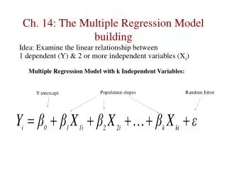
Testing the Strength of Multiple Regression Model: Are Any X's Useful in Predicting Y?
250 likes | 352 Vues
Test to determine if at least one factor (x) is useful in predicting y based on overall variability measurements. Calculating F-statistic, degrees of freedom, and p-value. Interpreting results to identify significant variables influencing the model.

Testing the Strength of Multiple Regression Model: Are Any X's Useful in Predicting Y?
E N D
Presentation Transcript
TESTING THE STRENGTH OF THE MULTIPLE REGRESSION MODEL
Test 1: Are Any of the x’s Useful in Predicting y? We are asking: Can we conclude at least one of the ’s (other than 0) 0? H0: 1 = 2 = 3 = 4 = 0 HA: At least one of these ’s 0 = .05
Idea of the Test • Measure the overall “average variability” due to changes in the x’s • Measure the overall “average variability” that is due to randomness (error) • If the overall “average variability” due to changes in the x’s IS A LOT LARGER than “average variability” due to error, we conclude at least is non-zero, i.e. at least one factor (x) is useful in predicting y
“Total Variability” • Just like with simple linear regression we have total sum of squares due to regression SSR , and total sum of squares due to error, SSE, which are printed on the EXCEL output. • The formulas are a more complicated (they involve matrix operations)
“Average Variability” • “Average variability” (Mean variability) for a group is defined as the Total Variability divided by the degrees of freedom associated with that group: • Mean Squares Due to Regression MSR = SSR/DFR • Mean Squares Due to Error MSE = SSE/DFE
Degrees of Freedom • Total number of degrees of freedom DF(Total) always = n-1 • Degrees of freedom for regression (DFR) = the number of factors in the regression (i.e. the number of x’s in the linear regression) • Degrees of freedom for error (DFE) = difference between the two = DF(Total) -DFR
The F-Statistic • The F-statistic is defined as the ratio of two measures of variability. Here, • Recall we are saying if MSR is “large” compared to MSE, at least one β ≠ 0. • Thus if F is “large”, we draw the conclusion is that HA is true, i.e. at least one β ≠ 0.
The F-test • “Large” compared to what? • F-tables give critical values for given values of • TEST: REJECT H0 (Accept HA) if: F = MSR/MSE > F,DFR,DFE
RESULTS • If we do not get a large F statistic • We cannot conclude that any of the variables in this model are significant in predicting y. • If we do get a large F statistic • We can conclude at least one of the variables is significant for predicting y . • NATURAL QUESTION -- • WHICH ONES?
DFR = #x’s DFE = Total DF- DFR Total DF = n-1 SSR SSE Total SS = (yi - )2
MSR = SSR/DFR MSE = SSE/DFE F = MSR/MSE P-value for the F test
Results • We see that the F statistic is 20.89762 • This would be compared to F.05,3,34 • From the F.05 Table, the value of F.05,3,34 is not given. • But F.05,3,30 = 2.92 and F.05,3,40 = 2.84. • And 20.89762 > either of these numbers. • The actual value of F.05,3,34 can be calculated by Excel by FINV(.05,3,34) = 2.882601 • USE SIGNIFICANCE F • This is the p-value for the F-Test • Significance F = 7.46 x 10-8 = .0000000746 < .05 • Can conclude that at least one x is useful in predicting y
Test 2: Which Variables Are Significant IN THIS MODEL? • The question we are asking is, “taking all the other factors (x’s) into consideration, does a change in a particular x (x3, say) value significantly affect y. • This is another hypothesis test (a t-test). • To test if the age of the house is significant: H0: 3 = 0 (x3 is not significant in this model) HA: 3 0 (x3 is significant in this model)
The t-test for a particular factor IN THIS MODEL • Reject H0 (Accept HA) if:
t-value for test of 3 = 0 p-value for test of 3 = 0
Reading Printout for the t-test • Simply look at the p-value • p-value for 3 = 0 is .02194 < .05 • Thus the age of the house is significant in this model • The other variables • p-value for 1 = 0 is .0000839 < .05 • Thus square feet is significant in this model • p-value for 2 = 0 is .15503 > .05 • Thus the land (acres) is not significant in this model
Does A Poor t-value Imply the Variable is not Useful in Predicting y? • NO • It says the variable is not significant IN THIS MODEL when we consider all the other factors. • In this model – land is not significant when included with square footage and age. • But if we would have run this model without square footage we would have gotten the output on the next slide.
p-value for land is .00000717. In this model Land is significant.
Can it even happen that F says at least one variable is significant, but none of the t’s indicate a useful variable? • YES EXAMPLES IN WHICH THIS MIGHT HAPPEN: • Miles per gallon vs. horsepower and engine size • Salary vs. GPA and GPA in major • Income vs. age and experience • HOUSE PRICE vs. SQUARE FOOTAGE OF HOUSE AND LAND • There is a relation between the x’s – • Multicollinearity
Approaches That Could Be Used When Multicollinearity Is Detected • Eliminate some variables and run again • Stepwise regression This is discussed in a future module.
Test 3 --What Proportion of the Overall Variability in y Is Due to Changes in the x’s? R2 • R2 = .442197 • Overall 44% of the total variation in sales price is explained by changes in square footage, land, and age of the house.
What is Adjusted R2? • Adjusted R2 adjusts R2 to take into account degrees of freedom. • By assuming a higher order equation for y, we can force the curve to fit this one set of data points in the model – eliminating much of the variability (See next slide). • But this is not what is going on! R2 might be higher – but adjusted R2 might be much lower • Adjusted R2 takes this into account • Adjusted R2 = 1-MSE/SST
Scatterplot This is not what is really going on
Review • Are any of the x’s useful in predicting y IN THIS MODEL • Look at p-value for F-test – Significance F • F = MSR/MSE would be compared to F,DFR,DFE • Which variables are significant in this model? • Look at p-values for the individual t-tests • What proportion of the total variance in y can be explained by changes in the x’s? • R2 • Adjusted R2 takes into account the reduced degrees of freedom for the error term by including more terms in the model
4 Places to Look on Excel Printout 4- R2 What proportion of y can be explained by changes in x? 2- Significance F Are any variables useful? 3- p-values for t-tests Which variables are significant in this model? 1-regression equation