The Simple Regression Model
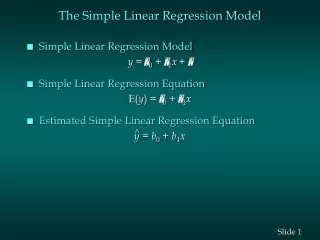
The Simple Regression Model. y = b 0 + b 1 x + u. Some Terminology. In the simple linear regression model, where y = b 0 + b 1 x + u , we typically refer to y as the Dependent Variable, or Left-Hand Side Variable, or Explained Variable, or. Some Terminology.

The Simple Regression Model
E N D
Presentation Transcript
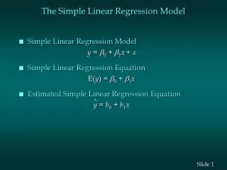
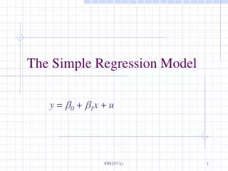
The Simple Regression Model y = b0 + b1x + u FIN357 Li
Some Terminology • In the simple linear regression model, where y = b0 + b1x + u, we typically refer to y as the • Dependent Variable, or • Left-Hand Side Variable, or • Explained Variable, or FIN357 Li
Some Terminology • we typically refer to x as the • Independent Variable, or • Right-Hand Side Variable, or • Explanatory Variable, or • Regressor, or • Control Variables FIN357 Li
A Simple Assumption • The average value of u, the error term, in the population is 0. That is, • E(u) = 0 FIN357 Li
We also assume • E(u|x) = 0 • E(y|x) = b0 + b1x FIN357 Li
E(y|x) as a linear function of x, where for any x the distribution of y is centered about E(y|x) y f(y) . E(y|x) = b0 + b1x . x1 x2 FIN357 Li
Ordinary Least Squares (OLS) • Let {(xi,yi): i=1, …,n} denote a random sample of size n from the population • For each observation in this sample, it will be the case that • yi = b0 + b1xi + ui FIN357 Li
Population regression line, sample data points and the associated error terms y E(y|x) = b0 + b1x . y4 { u4 . u3 y3 } . y2 u2 { u1 . } y1 x2 x1 x4 x3 x FIN357 Li
Basic idea of regression is to estimate the population parameters from a sample • Intuitively, OLS is fitting a line through the sample points such that the sum of squared residuals is as small as possible. • The residual, û, is an estimate of the error term, u, and is the difference between the fitted line (sample regression function) and the sample point FIN357 Li
Sample regression line, sample data points and the associated estimated error terms (residuals) y . y4 { û4 . û3 y3 } . y2 û2 { û1 } . y1 x2 x1 x4 x3 x FIN357 Li
One approach to estimate coefficients • Given the intuitive idea of fitting a line, we can set up a formal minimization problem • That is, we want to choose our parameters such that we minimize the following: FIN357 Li
Summary of OLS slope estimate • The slope estimate is the sample covariance between x and y divided by the sample variance of x • If x and y are positively correlated, the slope will be positive • If x and y are negatively correlated, the slope will be negative FIN357 Li
Algebraic Properties of OLS: in English • The sum of the OLS residuals is zero • Thus, the sample average of the OLS residuals is zero as well • The sample covariance between the regressors and the OLS residuals is zero • The OLS regression line always goes through the mean of the sample FIN357 Li
More terminology FIN357 Li
Notations Alert • The notation SSR (Sum of Squared Residuals) in this handout and my other lecture slides= ESS (Error Sum of Squares) in our textbook. • The notation SSE (Sum of Squared Explained) in this handout and my other lecture slides = RSS (Regressed Sum of Squares) in our textbook. FIN357 Li
Goodness-of-Fit • How do we think about how well our sample regression line fits our sample data? • Can compute the fraction of the total sum of squares (SST) that is explained by the model, call this the R-squared of regression • R2 = SSE/SST = 1 – SSR/SST FIN357 Li
OLS regressions • Now that we’ve derived the formula for calculating the OLS estimates of our parameters, you’ll be happy to know you don’t have to compute them by hand • Regressions in GRETL are very simple. • Have you installed the software yet? FIN357 Li
Under some conditions, OLS esimated coefficients are unbiased. FIN357 Li
Unbiasedness Summary • The OLS estimates of b1 and b0 are unbiased • Remember unbiasedness is a description of the estimator – in a given sample we may be “near” or “far” from the true parameter FIN357 Li
Variance of the OLS Estimators • Now we know that the sampling distribution of our estimated coefficient is centered around the true parameter • Want to think about how spread out this distribution is • Assume Var(u|x) =Var(u) = s2 FIN357 Li
Variance of OLS estimators • s2 is called the error variance • s, the square root of the error variance is called the standard deviation of the error • E(y|x)=b0 + b1x and Var(y|x) = s2 FIN357 Li
Variance of OLS estimator FIN357 Li
Variance of OLS Summary • The larger the error variance, s2, the larger the variance of the slope estimate • The larger the variability in the xi, the smaller the variance of the slope estimate • Problem that the error variance is unknown FIN357 Li
Estimating the Error Variance • We don’t know what the error variance, s2, is, because we don’t observe the errors, ui • What we observe are the residuals, ûi • We can use the residuals to form an estimate of the error variance FIN357 Li
Estimating the Error Variance FIN357 Li
Estimating Standard Error of coefficients Estimate FIN357 Li