
SlideServe
Menu
Préférences
© SlideServe · v2026

The Simple Linear Regression Model

cchaves avatar
12 diapositives · 310 Views · Jan 03, 2020

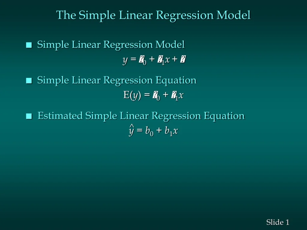
The Simple Linear Regression Model. Simple Linear Regression Model y =  0 +  1 x +  Simple Linear Regression Equation E( y ) =  0 +  1 x Estimated Simple Linear Regression Equation y = b 0 + b 1 x. ^. Least Squares Method. Least Squares Criterion where:
The Simple Linear Regression Model - slide 1
01 / 12The Simple Linear Regression Model
1 / 17

Télécharger la présentation

The Simple Linear Regression Model
Une image / un lien ci-dessous est fourni (tel quel) pour télécharger la présentation

Politique de téléchargement : le contenu du site vous est fourni TEL QUEL pour votre information et votre usage personnel ; il ne peut être vendu, concédé sous licence ni partagé sur d’autres sites sans l’accord de son auteur.Le contenu vous est fourni TEL QUEL, pour votre information et votre usage personnel uniquement. Téléchargez la présentation en cliquant sur ce lien. Lors du téléchargement, si vous ne parvenez pas à télécharger une présentation, l’éditeur a peut-être supprimé le fichier de son serveur.Pendant le téléchargement, si vous ne parvenez pas à obtenir une présentation, le fichier a peut-être été supprimé par l’éditeur.

F I N

Plus de contenu associé

Transcription de la présentation
  1. The Simple Linear Regression Model • Simple Linear Regression Model y = 0 + 1x+  • Simple Linear Regression Equation E(y) = 0 + 1x • Estimated Simple Linear Regression Equation y = b0 + b1x ^

  2. Least Squares Method • Least Squares Criterion where: yi = observed value of the dependent variable for the ith observation yi = estimated value of the dependent variable for the ith observation ^

  3. ^ ^ The Coefficient of Determination • Relationship Among SST, SSR, SSE SST = SSR + SSE • Coefficient of Determination r2 = SSR/SST where: SST = total sum of squares SSR = sum of squares due to regression SSE = sum of squares due to error

  4. The Correlation Coefficient • Sample Correlation Coefficient where: b1 = the slope of the estimated regression equation

  5. Model Assumptions • Assumptions About the Error Term  • The error  is a random variable with mean of zero. • The variance of  , denoted by  2, is the same for all values of the independent variable. • The values of  are independent. • The error  is a normally distributed random variable.

  6. Testing for Significance • To test for a significant regression relationship, we must conduct a hypothesis test to determine whether the value of b1 is zero. • Two tests are commonly used • t Test • F Test • Both tests require an estimate of s2, the variance of e in the regression model.

  7. Testing for Significance • An Estimate of s2 The mean square error (MSE) provides the estimate of s2, and the notation s2 is also used. s2 = MSE = SSE/(n-2) where:

  8. Testing for Significance • An Estimate of s • To estimate s we take the square root of s 2. • The resulting s is called the standard error of the estimate.

  9. Testing for Significance: t Test • Hypotheses H0: 1 = 0 Ha: 1 = 0 • Test Statistic • Rejection Rule Reject H0 if t < -tor t > t where tis based on a t distribution with n - 2 degrees of freedom.

  10. Testing for Significance: F Test • Hypotheses H0: 1 = 0 Ha: 1 = 0 • Test Statistic F = MSR/MSE • Rejection Rule Reject H0 if F > F where F is based on an F distribution with 1 d.f. in the numerator and n - 2 d.f. in the denominator.

  11. Using the Estimated Regression Equationfor Estimation and Prediction • Confidence Interval Estimate of E(yp) • Prediction Interval Estimate of yp yp+t/2 sind where the confidence coefficient is 1 -  and t/2 is based on a t distribution with n - 2 d.f.

  12. ^ Residual Analysis • Residual for Observation i yi – yi • Standardized Residual for Observation i where: ^ ^ ^