The Simple Linear Regression Model
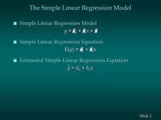
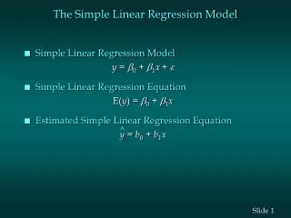
The Simple Linear Regression Model. Simple Linear Regression Model y = 0 + 1 x + Simple Linear Regression Equation E( y ) = 0 + 1 x Estimated Simple Linear Regression Equation y = b 0 + b 1 x. ^. 最小平方直線(最佳預測直線).

The Simple Linear Regression Model
E N D
Presentation Transcript
The Simple Linear Regression Model • Simple Linear Regression Model y = 0 + 1x+ • Simple Linear Regression Equation E(y) = 0 + 1x • Estimated Simple Linear Regression Equation y = b0 + b1x ^
最小平方直線(最佳預測直線) • 通過平面分佈圖資料點的直線中,使預測誤差平方和爲最小者即稱爲最小平方直線,而此方法即稱爲最小平方法(Least Square Method) • 何謂誤差平方和? 設 爲n個資料點,若以 做爲以X預測Y的直線,則當X=x1,預測值 與實際觀察的y1之差異 即稱爲預測誤差,誤差平方和即定義爲 求 使函數 f 爲最小時,由微積分解“極大或極小”方法。
最小平方直線 解此聯立方程組 可得 : 故最小平方直線為
Example: Reed Auto Sales • Simple Linear Regression Reed Auto periodically has a special week-long sale. As part of the advertising campaign Reed runs one or more television commercials during the weekend preceding the sale. Data from a sample of 6 previous sales are shown below. Number of TV AdsNumber of Cars Sold 1 14 3 24 2 18 1 17 3 27 2 22
Example: Reed Auto Sales • Slope for the Estimated Regression Equation b1 = 264 - (12)(122)/5 = 5 28 - (12)2/5 • y-Intercept for the Estimated Regression Equation b0 = 20.333 - 5(2) = 10.333 • Estimated Regression Equation y = 10.333 + 5x ^
Example: Reed Auto Sales • Scatter Diagram
^ ^ The Coefficient of Determination • Relationship Among SST, SSR, SSE SST = SSR + SSE • Coefficient of Determination r2 = SSR/SST where: SST = total sum of squares SSR = sum of squares due to regression SSE = sum of squares due to error
判定係數 • 定義: r2 = SSR/SST • 用以表示Y的變異數中已被X解釋的部分(比率) • 當r2 愈大時,表示最小平方直線愈精確 • 1- r2為總變異數(SST)中無法由X解釋的餘量(剩餘的比率) • 表示汽車銷售量的差異與變化有85.2%可由“廣告次數”這個因素來解釋(而有14.8%無法由“廣告次數”所解釋) Example: Reed Auto Sales r2 = SSR/SST = 100/117.333 = .852273
The Correlation Coefficient • Sample Correlation Coefficient where: b1 = the slope of the estimated regression equation
Example: Reed Auto Sales • Sample Correlation Coefficient The sign of b1 in the equation is “+”. rxy = +.923186
Model Assumptions • Assumptions About the Error Term • The error is a random variable with mean of zero. • The variance of , denoted by 2, is the same for all values of the independent variable. • The values of are independent. • The error is a normally distributed random variable.
Testing for Significance • To test for a significant regression relationship, we must conduct a hypothesis test to determine whether the value of b1 is zero. • Two tests are commonly used • t Test • F Test • Both tests require an estimate of s2, the variance of e in the regression model.
Testing for Significance • An Estimate of s2 The mean square error (MSE) provides the estimate of s2, and the notation s2 is also used. s2 = MSE = SSE/(n-2) where:
Testing for Significance • An Estimate of s • To estimate s we take the square root of s 2. • The resulting s is called the standard error of the estimate.
Testing for Significance: t Test • Hypotheses H0: 1 = 0 Ha: 1 = 0 • Test Statistic • Rejection Rule Reject H0 if t < -tor t > t where tis based on a t distribution with n - 2 degrees of freedom.
Example: Reed Auto Sales • t Test • Hypotheses H0: 1 = 0 Ha: 1 = 0 • Rejection Rule For = .05 and d.f. = 4, t.025 = 2.776 Reject H0 if t > 2.776 • Test Statistics t = 5/1.0408 = 4.804 • Conclusions Reject H0 • P-value 2P{T>4.804}=0.0086 <0.05 Reject H0
Confidence Interval for 1 • We can use a 95% confidence interval for 1 to test the hypotheses just used in the t test. • H0 is rejected if the hypothesized value of 1 is not included in the confidence interval for 1.
Confidence Interval for 1 • The form of a confidence interval for 1 is: where b1 is the point estimate is the margin of error is the t value providing an area of a/2 in the upper tail of a t distribution with n - 2 degrees of freedom
Example: Reed Auto Sales • Rejection Rule Reject H0 if 0 is not included in the confidence interval for 1. • 95% Confidence Interval for 1 = 5 2.776(1.0408) = 5 2.89 or 2.11 to 7.89 • Conclusion Reject H0
Testing for Significance: F Test • Hypotheses H0: 1 = 0 Ha: 1 = 0 • Test Statistic F = MSR/MSE • Rejection Rule Reject H0 if F > F where F is based on an F distribution with 1 d.f. in the numerator and n - 2 d.f. in the denominator.
Example: Reed Auto Sales • F Test • Hypotheses H0: 1 = 0 Ha: 1 = 0 • Rejection Rule • For = .05 and d.f. = 1, 4: F.05 = 7.709 • Reject H0 if F > 7.709. • Test Statistic • F = MSR/MSE = 100/4.333 = 23.077 • Conclusion • We can reject H0.
Some Cautions about theInterpretation of Significance Tests • Rejecting H0: b1 = 0 and concluding that the relationship between x and y is significant does not enable us to conclude that a cause-and-effect relationship is present between x and y. • Just because we are able to reject H0: b1 = 0 and demonstrate statistical significance does not enable us to conclude that there is a linear relationship between x and y.
Using the Estimated Regression Equationfor Estimation and Prediction • Confidence Interval Estimate of E(yp) • Prediction Interval Estimate of yp yp+t/2 sind where the confidence coefficient is 1 - and t/2 is based on a t distribution with n - 2 d.f. • is the standard error of the estimate of E(yp) sind is the standard error of individual estimate of
E(yp) 與yp估計式的變異數 • 的變異數: • 的變異數: • e的變異數: • 估計式的變異數: • 估計式的變異數:
Example: Reed Auto Sales • Point Estimation If 3 TV ads are run prior to a sale, we expect the mean number of cars sold to be: y = 10.333 + 5(3) = 25.333 cars • Confidence Interval for E(yp) 95% confidence interval estimate of the mean number of cars sold when 3 TV ads are run is: 25.333 + 3.730 = 21.603 to 29.063 cars • Prediction Interval for yp 95% prediction interval estimate of the number of cars sold in one particular week when 3 TV ads are run is: 25.333 + 6.878 = 18.455 to 32.211 cars ^