The Simple Linear Regression Model
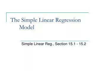
The Simple Linear Regression Model. Simple Linear Reg., Section 15.1 - 15.2. Regression Analysis. Examines the relationship between two continuous variables Postulates that the dependent variable, Y, is a linear function of the independent variable, X Allows us

The Simple Linear Regression Model
E N D
Presentation Transcript
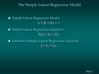
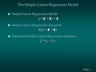
The Simple Linear Regression Model Simple Linear Reg., Section 15.1 - 15.2
Regression Analysis • Examines the relationship between two continuous variables • Postulates that the dependent variable, Y, is a linear function of the independent variable, X • Allows us • To measure the change in the dependent variable, Y, which corresponds to a given change in the independent or explanatory variable, X • To predict the dependent variable, Y, given a specific value of the independent variable, X PP 8
Examples • Earnings = f(Education) • Consumption = f(Income) • MPG = f(Weight of Vehicle) • Profits = f(Research Expenditures) • Yield of crop = f(fertilizer) PP 8
in X in Y Linear Relationships - Y = a + bX Y = 2 + 3X PP 8
Problem - The Relationship between the Percentage Immunized and the Mortality Rate • Investigate the relationship between the mortality rate for children under-5 years of age in a given country and the percentage of children who have been immunized against diptheria, pertussis, and tetanus (DPT) in that country • We have available a random sample of 20 countries • Let X represent the percentage of children immunized and Y represents the under-5 mortality rate • Mortality is the dependent variable, Y • Percentage immunized is the independent variable, X • The raw data, scatter diagram and computer output • Available at website as Handout for the Simple Regression Model PP 8
Y σy|x σy|x E(Y|X=20) E(Y|X=50) E(Y|X=80) σy|x 20 50 80 X The Population Regression Line • Select specific values for X (20, 50, 80) • At each value of immunization (X), there is a distribution of mortality rates (Y) • Conditional probability distribution of Y|X • Normally distributed • σy|x are homogeneous • E(Y|X) are linearly related to X PP 8
Y E(Y|X=20) E(Y|X=50) E(Y|X=80) 20 50 80 X The Population Regression Line • The population regression line – is the equation for a line • where E(Y|X) = is the mean value of Y for a given value of X • β0 and 1 are parameters - the coefficients of the equation and they are constants • β0 = the Y intercept for the population when X = 0 • 1 = the slope • interpreted as the change in the mean value of Y that corresponds to a one-unit change in X PP 8
Y E(Y|X=20) E(Y|X=50) E(Y|X=80) 20 50 80 X Population Regression Line • Sample data support claim of linearity • E(Y|X) = is the mean mortality rate for countries whose immunization is a given value of X • β0 = the mean mortality rate when immunization equals zero • 1 = tells us how the mean mortality rate changes for every one percentage point increase in the immunization rate • 1 can be positive or negative • If 1 > 0, then E(Y|X) increases as X increases • if 1 < 0, then E(Y|X) decreases as X increases PP 8
Population Regression Line • If I knew β0 and β1I could determine the E(Y|X) for a given X • The relationship would be deterministic • Implies the relationship between mean mortality rates and immunization rate is a perfect straight line • The relationship between individual mortality rates and immunization rates is not perfectly linear PP 8
Y E(Y|X=20) E(Y|X=50) E(Y|X=80) 20 50 80 X Population Regression Model Individual country values differ from the mean, E(Y|X) • For each specific immunization rate, there is a scattering of individual countries’ mortality rates around the mean mortality rate • To accommodate this scatter, the populationregression model iswhere i is the error term, i refers to the ith observation PP 8
yi εi X Regression Line and Regression Model • Error, εi, is the distance between the value of the observation, yi, and the mean value of Y given X • Compare the equation for the population model with the regression line E(Y|X) yi - E(Y|X) = εi PP 8
Error Term Y, Mortality The mortality rate for this country lies above the mean mortality rate for this value of the immunization rate. The sign of the error term will be ? ε> 0 The mortality rate for this country lies below the mean mortality rate for this level of x. The sign of the error term will be ? ε< 0 20 50 X, Immunity PP 8
yi εi X Assumptions of the Classical Linear Model • The conditional probability distribution of Y|X is also the distribution of ε|X E(ε) = 0 σε PP 8
Assumptions of the Classical Linear Model • First - The mean of the conditional probability distribution of Y lies on the true regression line • The E(εi) = 0 • Second - For any specified value of X, does not change • This assumption of equal standard deviations for each of the conditional probability distributions of Y|X is called homoskedasticity • The standard deviation of the error term does not change PP 8
Proof of First Assumption 0 and 1 are constants, population parameters. The E(Constant)=constant. xi is assumed to be a fixed specific value, and can be viewed as a constant and not a random variable. Therefore For this expression to equal the population regression line and for the line to predict mean values of Y for given X values, it most be true that the E(i) = 0 for all i. The mean error equals zero. PP 8
Assumptions of the Classical Linear Model • Third - The observations, yi, are statistically independent • If for x2 we observe y2 above the regression line, we do not expect that for x3, y3 will also be above the regression line • The reason the Y values would be consistently above the regression line is that the error terms are consistently positive • The error terms should be independent PP 8
Statistically Dependent Y Values εi Y event X event X PP 8
Plot of Residuals vs. X εi Plot the error term against the associated X value. Should observe no particular pattern. This implies statistical independence 0 X PP 8
yi εi X Assumptions of the Classical Linear Model • Fourth - To test null hypotheses, assume that the dependent variable Y is normally distributed • Really an assumption that the error term is normally distributed E(ε) = 0 σε PP 8
The Method of Least Squares • Now we have a sample and the problem is one of estimation • Estimate the unknown population regression line with a sample regression line • Given our scatter diagram of mortality against immunization rates, suppose we drew an arbitrary line through the scatter of points so that we could use this line to predict mortality for a given level of immunization • The line I draw would be different from the line you draw • My arbitrary line, which I will call my sample regression line, uses the following notation • where is the estimate of E(Y|X) • fitted value, predicted value • b0 is the estimate of 0 • and b1 is the estimate 1 PP 8
The Sample Regression Line - Using the “Eyeball” Method PP 8
The Sample Model • For the sample model • where eiis the sample estimate ofI • Compare the equation for the model with the regression line Model Regression equation PP 8
The Method of Least Squares • Each data point (xi,yi) lies some vertical difference from the arbitrary line • Label this distance, ei • yi is the observed outcome of Y for a particular value of X • is the predicted point on the fitted line • The distance ei is the residual • The estimate of the unknown error term in the population • Ideally we would like all the residuals to be equal to zero • This would imply that each point (xi ,yi) lies on the sample regression line • What we observe in the data would be identical to what we predict from our regression line • Since this is impossible we need some other criterion • We choose to minimize the residual yi ei xi PP 8
Minimizing the Error Sum of Squares Since we are interested in the distance and not the signs and since we want to minimize the residual term for all observations The goal is to minimize the SSE in terms of choosing b0 and b1. We use calculus to minimize PP 8
Minimizing the Error Sum of Squares We differentiate SSE with respect to b0and b1 and set the resulting two expressions equal to zero. We then have two equations in two unknowns. The first order conditions for a minimum are PP 8
Minimizing the Error Sum of Squares • These equations can be rearranged into the two Normal Equations: Solving for b0 and b1 Note: Sample regression line passes through the mean values of X and Y PP 8
where = mortality rate x = immunization rate Solving for the Sample Regression Coefficients • The sample size is 20 The sample regression line is PP 8
Predict • Use the sample regression line to predict the under 5 mortality rate for countries with some given value of immunization • Predict the mortality rate for countries with an immunization rate of 50% • 137 deaths per 1000 live births PP 8
Interpreting the Slope Coefficient • The slope coefficient tells us the average change in Y for every one unit change in X • The slope of -2.83 tells us that for every one percentage point increase in the immunization rate, the average under 5 mortality rate declines by 2.83 deaths per 1000 live births • The constant term suggests that there is a certain constant portion of the mortality rate that does not vary with immunization rates • One way to interpret the constant term is to say that it is the mean effect on Y of all the excluded variables for the relevant population PP 8
Online Homework - Chapter 15 Intro to Regression and Chapter 15 Simple Regression • CengageNOW twelfth assignment • CengageNOW thirteenth assignment PP 8
Properties of OLS Estimators • Each estimator, b0 and b1, is a linear combination of the observations, yi, they are linear estimators • If the yi’s are normally distributed and given that b1 is a linear combination of the yi’s, this implies that the estimator, b1, is normally distributed PP 8
Properties of OLS Estimators • Each estimator is unbiased • E(b1) =1E(b0) =0 • If we run many regressions, we expect, on average, to hit the true values of 0 and 1 • Among all the unbiased linear estimators, b0 and b1 have the lowest variance • The smaller the variance of an estimator, the better the chance of fitting the regression line close to the true population regression line • This is called the Gauss-Markov Theorem PP 8
normal normal E(b0) = β0 E(b1) = β1 Properties of OLS Estimators b0 b1 Estimators have the minimum variance of the class of linear unbiased estimators PP 8