Chapter 6 Further Inference in the Multiple Regression Model
1.66k likes | 1.96k Vues
Chapter 6 Further Inference in the Multiple Regression Model. Chapter Contents. 6.1 Joint Hypothesis Testing 6.2 The Use of Nonsample Information 6 .3 Model Specification 6 .4 Poor Data, Collinearity, and Insignificance 6 .5 Prediction.

Chapter 6 Further Inference in the Multiple Regression Model
E N D
Presentation Transcript
Chapter 6 Further Inference in the Multiple Regression Model
Chapter Contents • 6.1 Joint Hypothesis Testing • 6.2 The Use of Nonsample Information • 6.3 Model Specification • 6.4 Poor Data, Collinearity, and Insignificance • 6.5 Prediction
Economists develop and evaluate theories about economic behavior • Hypothesis testing procedures are used to test these theories • The theories that economists develop sometimes provide nonsample information that can be used along with the information in a sample of data to estimate the parameters of a regression model • A procedure that combines these two types of information is called restricted least squares
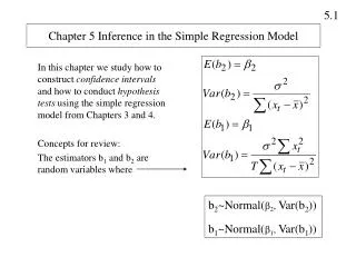
6.1 Joint Hypothesis Testing
6.1 Joint Hypothesis Testing 6.1 Testing Joint Hypotheses • A null hypothesis with multiple conjectures, expressed with more than one equal sign, is called a joint hypothesis • Example: Should a group of explanatory variables should be included in a particular model? • Example: Does the quantity demanded of a product depend on the prices of substitute goods, or only on its own price?
6.1 Joint Hypothesis Testing 6.1 Testing Joint Hypotheses • Both examples are of the form: • The joint null hypothesis in Eq. 6.1 contains three conjectures (three equal signs): β4 = 0, β5 = 0, and β6 = 0 • A test of H0 is a joint test for whether all three conjectures hold simultaneously Eq. 6.1
6.1 Joint Hypothesis Testing 6.1.1 Testing the Effect of Advertising: The F-Test • Consider the model: • Test whether or not advertising has an effect on sales – but advertising is in the model as two variables Eq. 6.2
6.1 Joint Hypothesis Testing 6.1.1 Testing the Effect of Advertising: The F-Test • Advertising will have no effect on sales if β3 = 0 and β4 = 0 • Advertising will have an effect if β3 ≠ 0 or β4 ≠ 0 or if both β3 and β4 are nonzero • The null hypotheses are:
6.1 Joint Hypothesis Testing 6.1.1 Testing the Effect of Advertising: The F-Test • Relative to the null hypothesis H0 : β3 = 0, β4 = 0 the model in Eq. 6.2 is called the unrestricted model • The restrictions in the null hypothesis have not been imposed on the model • It contrasts with the restricted model, which is obtained by assuming the parameter restrictions in H0 are true
6.1 Joint Hypothesis Testing 6.1.1 Testing the Effect of Advertising: The F-Test • When H0 is true, β3 = 0 and β4 = 0, and ADVERT and ADVERT2 drop out of the model • The F-test for the hypothesis H0 : β3 = 0, β4 = 0 is based on a comparison of the sums of squared errors (sums of squared least squares residuals) from the unrestricted model in Eq. 6.2 and the restricted model in Eq. 6.3 • Shorthand notation for these two quantities is SSEU and SSER, respectively Eq. 6.3
6.1 Joint Hypothesis Testing 6.1.1 Testing the Effect of Advertising: The F-Test • The F-statistic determines what constitutes a large reduction or a small reduction in the sum of squared errors where J is the number of restrictions, N is the number of observations and K is the number of coefficients in the unrestricted model Eq. 6.4
6.1 Joint Hypothesis Testing 6.1.1 Testing the Effect of Advertising: The F-Test • If the null hypothesis is true, then the statistic F has what is called an F-distribution with J numerator degrees of freedom and N - K denominator degrees of freedom • If the null hypothesis is not true, then the difference between SSER and SSEU becomes large • The restrictions placed on the model by the null hypothesis significantly reduce the ability of the model to fit the data
6.1 Joint Hypothesis Testing 6.1.1 Testing the Effect of Advertising: The F-Test • The F-test for our sales problem is: • Specify the null and alternative hypotheses: • The joint null hypothesis is H0 : β3 = 0, β4 = 0. The alternative hypothesis is H0 : β3 ≠ 0 or β4 ≠ 0 both are nonzero • Specify the test statistic and its distribution if the null hypothesis is true: • Having two restrictions in H0means J = 2 • Also, recall that N = 75:
6.1 Joint Hypothesis Testing 6.1.1 Testing the Effect of Advertising: The F-Test • The F-test for our sales problem is (Continued): • Set the significance level and determine the rejection region • Calculate the sample value of the test statistic and, if desired, the p-value • The corresponding p-value is p = P(F(2, 71)> 8.44) = 0.0005
6.1 Joint Hypothesis Testing 6.1.1 Testing the Effect of Advertising: The F-Test • The F-test for our sales problem is (Continued): • State your conclusion • Since F = 8.44 > Fc = 3.126, we reject the null hypothesis that both β3 = 0 and β4 = 0, and conclude that at least one of them is not zero • Advertising does have a significant effect upon sales revenue
6.1 Joint Hypothesis Testing 6.1.2 Testing the Significance of the Model • Consider again the general multiple regression model with (K - 1) explanatory variables and K unknown coefficients • To examine whether we have a viable explanatory model, we set up the following null and alternative hypotheses: Eq. 6.5 Eq. 6.6
6.1 Joint Hypothesis Testing 6.1.2 Testing the Significance of the Model • Since we are testing whether or not we have a viable explanatory model, the test for Eq. 6.6 is sometimes referred to as a test of the overall significance of the regression model. • Given that the t-distribution can only be used to test a single null hypothesis, we use the F-test for testing the joint null hypothesis in Eq. 6.6
6.1 Joint Hypothesis Testing 6.1.2 Testing the Significance of the Model • The unrestricted model is that given in Eq. 6.5 • The restricted model, assuming the null hypothesis is true, becomes: Eq. 6.7
6.1 Joint Hypothesis Testing 6.1.2 Testing the Significance of the Model • The least squares estimator of β1 in this restricted model is: • The restricted sum of squared errors from the hypothesis Eq. 6.6 is:
6.1 Joint Hypothesis Testing 6.1.2 Testing the Significance of the Model • Thus, to test the overall significance of a model, but not in general, the F-test statistic can be modified and written as: Eq. 6.8
6.1 Joint Hypothesis Testing 6.1.2 Testing the Significance of the Model • For our problem, note: • We are testing: • If H0 is true:
6.1 Joint Hypothesis Testing 6.1.2 Testing the Significance of the Model • For our problem, note (Continued): • Using a 5% significance level, we find the critical value for the F-statistic with (3,71) degrees of freedom is Fc = 2.734. • Thus, we reject H0if F ≥ 2.734. • The required sums of squares are SST = 3115.482 and SSE = 1532.084 which give an F-value of: • p-value = P(F ≥ 24.459) = 0.0000
6.1 Joint Hypothesis Testing 6.1.2 Testing the Significance of the Model • For our problem, note (Continued): • Since 24.459 > 2.734, we reject H0and conclude that the estimated relationship is a significant one • Note that this conclusion is consistent with conclusions that would be reached using separate t-tests for the significance of each of the coefficients
6.1 Joint Hypothesis Testing • We used the F-test to test whether β3 = 0 and β4 = 0 in: • Suppose we want to test if PRICE affects SALES 6.1.3 Relationship Between the t- and F-Tests Eq. 6.9 Eq. 6.10
6.1 Joint Hypothesis Testing • The F-value for the restricted model is: • The 5% critical value is Fc = F(0.95, 1, 71) = 3.976 • We reject H0 : β2 = 0 6.1.3 Relationship Between the t- and F-Tests
6.1 Joint Hypothesis Testing • Using the t-test: • The t-value for testing H0: β2 = 0 against H1: β2 ≠ 0 is t = 7.640/1.045939 = 7.30444 • Its square is t = (7.30444)2 = 53.355, identical to the F-value 6.1.3 Relationship Between the t- and F-Tests
6.1 Joint Hypothesis Testing • The elements of an F-test • The null hypothesis H0consists of one or more equality restrictions on the model parameters βk • The alternative hypothesis states that one or more of the equalities in the null hypothesis is not true • The test statistic is the F-statistic in (6.4) • If the null hypothesis is true, F has the F-distribution with J numerator degrees of freedom and N - K denominator degrees of freedom • When testing a single equality null hypothesis, it is perfectly correct to use either the t- or F-test procedure: they are equivalent 6.1.3 Relationship Between the t- and F-Tests
6.1 Joint Hypothesis Testing 6.1.4 More General F-Tests • The conjectures made in the null hypothesis were that particular coefficients are equal to zero • The F-test can also be used for much more general hypotheses • Any number of conjectures (≤ K) involving linear hypotheses with equal signs can be tested
6.1 Joint Hypothesis Testing 6.1.4 More General F-Tests • Consider the issue of testing: • If ADVERT0 = $1,900 per month, then: or Eq. 6.11
6.1 Joint Hypothesis Testing 6.1.4 More General F-Tests • Note that when H0 is true, β3 = 1 – 3.8β4 so that: or Eq. 6.12
6.1 Joint Hypothesis Testing 6.1.4 More General F-Tests • The calculated value of the F-statistic is: • For α = 0.05, the critical value is Fc = 3.976 Since F = 0.9362 < Fc = 3.976, we do not reject H0 • We conclude that an advertising expenditure of $1,900 per month is optimal is compatible with the data
6.1 Joint Hypothesis Testing 6.1.4 More General F-Tests • The t-value is t = 0.9676 • F = 0.9362 is equal to t2 = (0.9676)2 • The p-values are identical:
6.1 Joint Hypothesis Testing 6.1.4a One-tail Test • Suppose we have: • In this case, we can no longer use the F-test • Because F = t2, the F-test cannot distinguish between the left and right tails as is needed for a one-tail test • We restrict ourselves to the t-distribution when considering alternative hypotheses that have inequality signs such as < or > Eq. 6.13
6.1 Joint Hypothesis Testing 6.1.5 Using Computer Software • Most software packages have commands that will automatically compute t- and F-values and their corresponding p-values when provided with a null hypothesis • These tests belong to a class of tests called Wald tests
6.1 Joint Hypothesis Testing 6.1.5 Using Computer Software • Suppose we conjecture that: • We formulate the joint null hypothesis: • Because there are J = 2 restrictions to test jointly, we use an F-test • A t-test is not suitable
6.2 The Use of Nonsample Information
6.2 The Use of Nonsample Information • In many estimation problems we have information over and above the information contained in the sample observations • This nonsample information may come from many places, such as economic principles or experience • When it is available, it seems intuitive that we should find a way to use it
6.2 The Use of Nonsample Information • Consider the log-log functional form for a demand model for beer: • This model is a convenient one because it precludes infeasible negative prices, quantities, and income, and because the coefficients β2, β3, β4, and β5are elasticities Eq. 6.14
6.2 The Use of Nonsample Information • A relevant piece of nonsample information can be derived by noting that if all prices and income go up by the same proportion, we would expect there to be no change in quantity demanded • For example, a doubling of all prices and income should not change the quantity of beer consumed • This assumption is that economic agents do not suffer from ‘‘money illusion’’
6.2 The Use of Nonsample Information • Having all prices and income change by the same proportion is equivalent to multiplying each price and income by a constant, say λ: Eq. 6.15
6.2 The Use of Nonsample Information • To have no change in ln(Q) when all prices and income go up by the same proportion, it must be true that: • We call such a restriction nonsample information Eq. 6.16
6.2 The Use of Nonsample Information • To estimate a model, start with: • Solve the restriction for one of the parameters, say β4: Eq. 6.17
6.2 The Use of Nonsample Information • Substituting gives: Eq. 6.18
6.2 The Use of Nonsample Information • To get least squares estimates that satisfy the parameter restriction, called restricted least squares estimates, we apply the least squares estimation procedure directly to the restricted model: Eq. 6.19
6.2 The Use of Nonsample Information • Let the restricted least squares estimates in Eq. 6.19 be denoted by b*1, b*2, b*3, and b*5 • To obtain an estimate for β4, we use the restriction: • By using the restriction within the model, we have ensured that the estimates obey the constraint:
6.2 The Use of Nonsample Information • Properties of this restricted least squares estimation procedure: • The restricted least squares estimator is biased, unless the constraints we impose are exactly true • The restricted least squares estimator is that its variance is smaller than the variance of the least squares estimator, whether the constraints imposed are true or not
6.3 Model Specification
6.3 Model Specification • In any econometric investigation, choice of the model is one of the first steps • What are the important considerations when choosing a model? • What are the consequences of choosing the wrong model? • Are there ways of assessing whether a model is adequate?
6.3 Model Specification 6.3.1 Omitted Variables • It is possible that a chosen model may have important variables omitted • Our economic principles may have overlooked a variable, or lack of data may lead us to drop a variable even when it is prescribed by economic theory
6.3 Model Specification 6.3.1 Omitted Variables • Consider the model: Eq. 6.20