Download
1 / 22
220 likes | 267 Vues
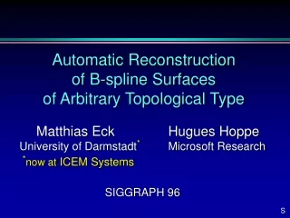
This research paper discusses an automatic procedure for reconstructing B-spline surfaces of arbitrary topological type with G1 continuity and error tolerance. It outlines a 5-step procedure including parametrization, B-spline fitting, and adaptive refinement, providing analysis and future directions for improvement.

E N D
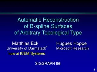
Automatic Reconstructionof B-spline Surfacesof Arbitrary Topological Type Matthias Eck Hugues Hoppe University of Darmstadt* Microsoft Research SIGGRAPH 96 *now at ICEM Systems S
Surface reconstruction • Reverse engineering • Traditional design (wood,clay) • Virtual environments pointsP surface S surfacereconstruction
arbitrary B-spline [Krishnamurthy-96], [Milroy-etal95], ... Previous work surface topological type simple arbitrary meshes [Schumaker93], … [Hoppe-etal92], [Turk-Levoy94], ... implicit [Sclaroff-Pentland91], ... [Moore-Warren91], [Bajaj-etal95] subdivision - [Hoppe-etal94] smooth B-spline [Schmitt-etal86], [Forsey-Bartels95],... [Krishnamurthy-96], [Milroy-etal95],...
Problem statement • automatic procedure • surface of arbitrary topological type • S smooth ÞG1 continuity • error tolerance e reconstructionprocedure points P B-spline surface S
N Þ require network N of B-spline patches 3 Difficulties: 1) Obtaining N 2) Parametrizing P over N 3) Fitting with G1 continuity Main difficulties S: arbitrary topological type singleB-spline patch
Comparison with previous talk Krishnamurthy- Levoy Eck- Hoppe patch network N curve painting automatic partitioning parametrizedP hierarchical remeshing harmonic maps continuity stitching step G1 construction
Overview of our procedure 5 steps: 1) Initial parametrization of P over mesh M0 2) Reparam. over triangular complex KD 3) Reparam. over quadrilateral complex Kÿ 4) B-spline fitting 5) Adaptive refinement
(1) Find an initial parametrization a) construct initial surface: dense mesh M0 b) parametrize P over M0 Using: [Hoppe-etal92] [Hoppe-etal93] P M0
a) partition M0 into triangular regions b) parametrize each region using a harmonic map partitioned M0 base mesh KD (2) Reparametrize over domain KD • Use parametrization scheme of [Eck-etal95]: M0
Harmonic map [Eck-etal95] planar triangle triangular region map minimizing metric distortion
Reparametrize points M0 KD using harmonic maps
(3) Reparametrize over Kÿ • Merge faces of KD pairwise • cast as graph optimization problem KD Kÿ
harmonicmap two D regions planar square • For each pair of adjacent D regions,let edge cost = harmonic map “distortion” • Solve MAX-MIN MATCHING graph problem Graph optimization
Kÿ reparametrize P using harmonic maps
(4) B-spline fitting • Use surface spline scheme of [Peters94]: • G1 surface • tensor product B-spline patches • low degree • Other similar schemes • [Loop94],[Peters96], …
Fitting using [Peters94] scheme affine Kÿ Mx optimization Overview of [Peters94] scheme 2 Doo-Sabinsubdiv. affine construction B-splinebases Mc Mx df S (Details: linear constraints, reprojection, fairing, …)
(5) Adaptively refine the surface • Goal: make P and S differ by no more than e • Strategy: adaptively refine Kÿ 4 facerefinement templates S# K# Kÿ e: 1.02% Þ 0.74%
Reconstruction results Sÿ P 20,000 points 29 patchese = 1.20% rms = 0.20%
Reconstruction results 29 patchese = 1.20% rms = 0.20% 156 patchese = 0.27% rms = 0.03%
Approximation results S0 P S# 70,000triangles 30,000points 153 patchese = 1.44% rms = 0.19%
Analysis Krishnamurthy- Levoy Eck- Hoppe patch network N curve painting automatic partitioning parametrizedP hierarchical remeshing harmonic maps continuity stitching step G1 construction refinement no yes displac. map yes no
Future work • Semi-automated layout of patch network • Allowing creases and corners in B-spline construction • Error bounds on surface approximation have: d(P,S)<e want: d(S0,S)<e


![Texture Synthesis on [Arbitrary Manifold] Surfaces](https://cdn2.slideserve.com/4198281/texture-synthesis-on-arbitrary-manifold-surfaces-dt.jpg)