Download
1 / 36
370 likes | 1.03k Vues
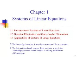
Solving [Specific Classes of] Linear Equations using Random Walks Haifeng Qian Sachin Sapatnekar x 1 x 2 : x n b 1 b 2 : b n a ii Row i = Definition of diagonal dominance Matrix A is diagonally dominant if a ii ij |a ij | Consider a system of linear equations

E N D
Solving [Specific Classes of] Linear Equations using Random Walks Haifeng Qian Sachin Sapatnekar
x1 x2 : xn b1 b2 : bn aii Row i = Definition of diagonal dominance • Matrix A is diagonally dominant if aiiij|aij| • Consider a system of linear equations • Can solve Ax = b rapidly using a random walk analogy if A is diagonally dominant (but not singular, of course!) (abbreviated as Ax = b)
Why do I care? • Diagonally dominant systems arise in several contexts in CAD (and in other fields) – for example, • Power grid analysis • VLSI Placement • ESD analysis • Thermal analysis • FEM/FDM analyses • Potential theory • The idea for random walk-based linear solvers has been around even in the popular literature • R. Hersh and R. J. Griego, “Brownian motion and potential theory,” Scientific American, pp. 67-74, March 1969. • P. G. Doyle and J. L. Snell, Random walks and electrical networks, Mathematical Association of America, Washington DC, 1984. http://math.dartmouth.edu/~doyle/docs/walks/walks.pdf
Dirichlet’s problem • Dirichlet problem: an example – thermal analysis • Given a body of arbitrary shape, and complete information about temperature on the surface: find termperature at an internal point • Temperature is a harmonic function: temperature at a point depends on average temperature of surrounding points • Shizuo Kakutani (1944) – solution of Dirichlet problem • Brownian motion starting from a point (say, a) • Take an award T = temperature of first boundary point hit • Find E[T] a b
Equations Random event(s) Variables Expectation of random variables Approximate solution Average of random samples Stochastic solvers Stochastic solver methodology
2 g2 g1 g3 x 3 1 g4 Ix 4 Example: Power grid analysis • Network of resistors and current sources • The equation at node x is Alternatively
∑ 1 Mapping this to the random walk “game” • Solving a grid amounts to solving, at each node:or
$ Home Home Home Random walk overview • Given: • A network of roads • A motel at eachintersection • A set of homes • Random walk • Walk one (randomlychosen) road every day • Stay the night at a motel (pay for it!) • Keep going until reaching home • Win a reward for reaching home! • Problem: find the expected amount of money in the end as a function of the starting node x
4 px,4 x 1 3 px,1 px,3 px,2 2 Random walk overview • For every node
Linear equation set Random walk game M walks from i-th node Take average This yields xi Random walk overview
$0 $1 0.33 0.33 +$0.13 -$0.2 -$ 0.05 +$ 0.45 A A 0.44 0.44 0.67 0.67 $1 $0 $0 $1 B B D D 0.2 0.2 0.44 0.44 0.5 0.5 0.8 0.8 -$0.04 +$0.76 0.5 0.5 0.12 0.12 -$0.022 -$0.022 C C Example • Solution: xA=0.6 xB=0.8 xC=0.7 xD=0.9
Average $0 -$0.284 $0 -$0.222 $0 -$0.222 -$0.422 -$0.2 $0.8 $0.578 $0.382 $0.444 $0.738 -$0.618 -$0.556 -$0.262 $0 $0 $0 -$0.516 -$0.222 -$0.222 -$0.578 -$0.262 -$0.2 -$0.2 -$0.494 -$0.422 -$0.2 -$0.556 -$0.2 -$0.484 -$0.2 -$0.506 -$0.222 -$0.444 $0.728 -$0.272 0.6 0.33 A 0.44 0.67 B D 0.2 0.44 0.5 0.8 0.5 0.12 C Play the game $1 Pocket: -$0.2 $1 $1 -$0.05 -$0.04 -$0.022 • Walk results: $0.578 $0.444 $0.8 $0.728 …… $0.738 $0.382
Start Start Reusing computations: avoiding repeated walks(When solving for all xi values) New home Previously calculated node Benefit: more and more homes shorter and shorter walks one walk = average of multiple walks Qian et al., DAC2003
Reusing computations: “Journey record”(when solving for multiple right hand sides) Keep a record: motel/award list New RHS: Ax = b2 Update motel prices, award values Use the record: pay motels, receive awards New solution Benefit: no more walks only feasible after trick#1 Qian et al., DAC2003
Error vs. runtime tradeoffs • Industrial circuit • 70729 nodes, 31501 bottom-layer nodes • VDD net true voltage range 1.1324—1.1917
Random walk overview • Advantage • Locality: solve single entry • Weakness • Error ~ M-0.5 • 3% error to be faster than direct/iterative solvers
Example application: Power grid analysis • Exact DC analysis: Solve GX = E • Very expensive to solve for millions of nodes, eventually prohibitive • Simple observations: • VDD and GND pins all over chip surface (C4 connections) • Most current drawn from “nearby” connections
Current techniques • Preconditioning • Popular choice: Incomplete LU • Placement/thermal matrices • Symmetric positive definite • Popular choice: ICCG with • Different ordering • Different dropping rules
Current techniques done done • Rules • Pattern • Min value • Size limit
stochastic precondi-tioning adopt an iterative scheme Iterative Solver The Hybrid Solver Stochastic Solver Stochastic preconditioning • Special case today • Symmetric • Positive diagonal entries • Negative off-diagonal entries • Irreducibly diagonally dominant • These are sufficient, NOT necessary, conditions
Stochastic Solver New solution: Sequential Monte Carlo Stochastic Solver approx. solve error & residual approx. solve Benefit: ||r||2<<||b||2 ||y||2<<||x||2 same relative error = lower absolute error A. W. Marshall 1956, J. H. Halton 1962
Keep a record: motel/award list Stochastic Solver New RHS: Ax = b2 Update motel prices, award values Stochastic Solver Use the record: pay motels, receive awards New solution New solution: This is computationally easy! Can show that this amounts to preconditioned Gauss-Jacobi So - why G-J? Why not CG/BiCG/MINRES/GMRES
Solver using the record What’s on the journey record? Row i These are “UL” factors. Relation to LU factors? Just a matrix reordering!
Recall LDL factorization • What we need for symmetric A • What we have • How to find ? • Easy – details omitted here • Easy extension to asymmetric matrices exists
Compare to existing ILU • Existing ILU • Gaussian elimination • Drop edges by pattern, value, size • Error propagation • A missing edge affects subsequent computation • Exacerbated for larger and denser matrices b2 b2 b1 b1 a b3 b3 b5 b5 b4 b4
Superior because … • Each row of L is independently calculated • No knowledge of other rows • Responsible for its own accuracy • No debt from other steps
Test setup • Quadratic placement instances • Set #1: matrices and rhs’s by an industrial placer • Set #2: matrices by UWaterloo placer on ISPD02 benchmarks, unit rhs’s • LASPACK: ICCG with ILU(0) • MATLAB: ICCG with ILUT • Approx. Min. Degree ordering • Tuned to similar factorization size • Same accuracy: • Complexity metric: # double-precision multiplications • Solving stage only
Physical runtimes on P4-2.8GHz • Reasonable preconditioning overhead • Less than 3X solving time • One-time cost, amortized over multiple solves
Newer results • Examples generated from Sparskit • Finite difference discretization of 3D Laplace’s equation under Dirichlet boundary conditions • S: #nonzeros in preconditioner (similar in all cases) • C1: Condition # of original matrix • C2: Condition # after split preconditioning Ex1 Ex2 Ex3 Ex4 Ex5 Ex6
Conclusion • Direct solver • Locality property • Reasonable for approximate solutions • Hybrid solver • Stochastically preconditioned iterative solver • Independent row/column estimates for LU factors • Better quality than same-size traditional ILU • Extension to non-diagonally dominant matrices? • Some pointers exist (see Haifeng Qian’s thesis) • Needs further work…
Thank you! • Downloads • Solver package http://www.ece.umn.edu/users/qianhf/hybridsolver • Thesis http://www-mount.ece.umn.edu/~sachin/Theses/HaifengQian.pdf
Thanks also (and especially) to… Haifeng Qian (He will pick up the 2006 ACM Oustanding Dissertation Award in Electronic Design Automation in San Diego next week)