Download
1 / 65
650 likes | 1.08k Vues
12. System of Linear Equations. Case Study. 12.1 System of Linear Equations. 12.2 Solving Equations by Inverses of Matrices. 12.3 Solving Equations by Cramer’s Rule. 12.4 Solving Equations by Gaussian Elimination. 12.5 Homogeneous Systems of Linear Equations. Chapter Summary.

E N D
12 System of Linear Equations Case Study 12.1 System of Linear Equations 12.2 Solving Equations by Inverses of Matrices 12.3 Solving Equations by Cramer’s Rule 12.4 Solving Equations by Gaussian Elimination 12.5 Homogeneous Systems of Linear Equations Chapter Summary
Since we know what chemicals are involved in the reaction, let us write down the balanced equation for this process. But we need to know the amount of each chemical first! Case Study In a Biology lesson, a group of students are doing experiments to study the process of photosynthesis. During the process, carbon dioxide (CO2) and water (H2O) would be converted into glucose (C6H12O6), and some oxygen (O2) is released: p CO2 q H2O r C6H12O6 s O2 where p, q, r and s are real numbers. In order to balance the equation, the numbers of atoms of carbon (C), oxygen (O) and hydrogen (H) should be the same on both sides of the equation. For example: Number of carbon atoms before the process p p 6r Number of carbon atoms after the process 6r
Case Study Chemical equation: p CO2 q H2O r C6H12O6 s O2 where p, q, r and s are real numbers. Number of C atoms before the process p p 6r Number of C atoms after the process 6r Number of O atoms before the process 2p + q 2p + q 6r + 2s Number of O atoms after the process 6r + 2s Number of H atoms before the process 2q 2q 12r Number of H atoms after the process 12r We can express the above details as a system of linear equations:
12.1 System of Linear Equations A system of m linear equations (or a linear system) in n unknowns x1, x2, x3, ¼, xn is a set of equations of the form The constants aijare called the coefficients of the system of linear equations. For example, is a system of two linear equations with three unknowns x, y and z.
Ax b, where , and . For example, can be expressed as . 12.1 System of Linear Equations In a system of linear equations, if there exists a set of numbers {N1, N2, …, Nn} satisfying all the equations, then the system is said to be solvable or consistent, and {N1, N2, …, Nn} is called a solution of the system of linear equations. Otherwise, the system is said to be non-solvable or inconsistent. The system of linear equations may be represented by the matrix equation Here, A is called the coefficient matrix, x is called the unknown matrix and (N1, N2, …, Nn)t is called the solution matrix.
12.2Solving Equations by Inverses of Matrices Suppose we have a system of linear equations of order 3: We can express the system in the matrix equation Ax b, where A is a 3 3 coefficient matrix. If A is non-singular, then the solution matrix x can be found by computing the inverse of A, and the solution is unique.
12.2Solving Equations by Inverses of Matrices Theorem 12.1 Let A be a square matrix. If A is non-singular, then the system of linear equations Ax b has a unique solution given by x A1b. Proof: If A is a non-singular matrix, then A1 exists. Axb (A1A)x A1b Ix A1b x A1b Therefore, the solution of Ax b exists. Now suppose Ax b has two solutions x1 and x2. Then Ax1b and Ax2 b. x1A1b and x2A1b. \x1x2 Therefore, the solution of Axb is unique.
Solve by the method of inverse matrix. Express the system of equations as ,where . \ A1 exists and 12.2Solving Equations by Inverses of Matrices Example 12.1T Solution: \ The unique solution of the system of linear equations is x 18, y 10.
Solve by the method of inverse matrix. Express the system of equations as where \ A1 exists and 12.2Solving Equations by Inverses of Matrices Example 12.2T Solution:
12.2Solving Equations by Inverses of Matrices We know that a square matrix A is non-singular if and only if|A| 0. Theorem 12.2 Let A be a square matrix. The system of linear equations Ax b has a unique solution if and only if |A| 0. This theorem can be used to test whether a system of linear equations has a unique solution. When |A| 0, A1 does not exist, so the method of inverse matrix cannot be applied. In this situation, either of the following cases will happen: 1. the system of equations does not have any solution, or 2. the system of equations has infinitely many solutions.
Determine the number of solutions to the following systems of linear equations. (a) (b) Consider 12.2Solving Equations by Inverses of Matrices Example 12.3T Solution: (a) Rewrite the system of equations as \ The system does not have a unique solution. Since (2) and (3) are the same, we say that equation (2) is redundant and the linear system has only one equation –x + 2y 1. Therefore, the system of linear equation has infinitely many solutions.
Consider 12.2Solving Equations by Inverses of Matrices Example 12.3T Determine the number of solutions to the following systems of linear equations. (a) (b) Solution: (b) Rewrite the system of equations as \ The system does not have a unique solution. (3) – (2): 0 5, which is impossible. Therefore, the system of linear equations has no solution.
Theorem 12.3 Cramer’s Rule of Order 2 Given a system of linear equations If the determinant of the coefficient matrix A is non-zero, the unique solution of the system is given by and 12.3Solving Equations by Cramer’s Rule Finding the inverse of the coefficient matrix is sometimes complicated, so in this section we will study how to use Cramer’s rule to solve a system of linear equations in a more convenient way.
Proof: From Theorem 12.1, if the determinant of the coefficient matrix A is non-zero, then xA1b, where x and b . For x A1b, we have . Definition of A1 12.3 Solving Equations by Cramer’s Rule If we express x1 and x2 in determinant form, we can obtain
Solve by Cramer’s rule. 12.3 Solving Equations by Cramer’s Rule Example 12.4T Solution: The determinant of the coefficient matrix \ The unique solution of the system of linear equations is
Theorem 12.4 Cramer’s Rule of Order 3 Given a linear system If the determinant of the coefficient matrix A is non-zero, the unique solution of the system is given by 12.3 Solving Equations by Cramer’s Rule For systems of linear equations of order 3, Cramer’s rule is stated as follows: Comparing Theorems 12.3 and 12.4, we can see that in both cases, the solution xj can be expressed as a fraction with |A| as the denominator, and the numerator is the determinant that replaces the elements in the jth column of A by bi’s.
Solve by Cramer’s rule. The determinant of the coefficient matrix 12.3 Solving Equations by Cramer’s Rule Example 12.5T Solution: \ The unique solution of the system of linear equations is
Although Cramer’s rule can be used to find the solution quickly, the solution is undefined when D|A| 0. 12.3 Solving Equations by Cramer’s Rule So it is only applicable when the coefficient matrix A is a non-singular matrix.
R2 R1 R2 R3 R1 R3 12.3 Solving Equations by Cramer’s Rule Example 12.6T Suppose we have a system of linear equations where a, b and c are real numbers. (a)If the system of linear equations has a unique solution, show that a, b and c are distinct and a + b + c 0. Solution: (a) The determinant of the coefficient matrix ∆
From the given equations, a 0, b 0 and c 0. 12.3 Solving Equations by Cramer’s Rule Example 12.6T Suppose we have a system of linear equations where a, b and c are real numbers. (a)If the system of linear equations has a unique solution, show that a, b and c are distinct and a + b + c 0. Solution: (a) ∵ The system of linear equations has a unique solution. \ D 0 i.e., abc(b – a)(c – a)(c – b)(a + b + c) 0 \a, b, c are distinct and a + b + c 0.
Take out the common factors R2 R1 R2 R3 R1 R3 12.3 Solving Equations by Cramer’s Rule Example 12.6T Suppose we have a system of linear equations where a, b and c are real numbers. (a)If the system of linear equations has a unique solution, show that a, b and c are distinct and a + b + c 0. (b)Solve the system of linear equations if it has a unique solution. Solution: (b)
12.3 Solving Equations by Cramer’s Rule Example 12.6T Suppose we have a system of linear equations where a, b and c are real numbers. (a)If the system of linear equations has a unique solution, show that a, b and c are distinct and a + b + c 0. (b)Solve the system of linear equations if it has a unique solution. Solution: (b)
12.3 Solving Equations by Cramer’s Rule Example 12.6T Suppose we have a system of linear equations where a, b and c are real numbers. (a)If the system of linear equations has a unique solution, show that a, b and c are distinct and a + b + c 0. (b)Solve the system of linear equations if it has a unique solution. Solution: The unique solution of the system of linear equations is (b)
12.4Solving Equations by Gaussian Elimination In the last two sections, we learnt how to solve systems of linear equations of order 2 and 3. However, those methods can only be applied when the coefficient matrix is a non-singular square matrix. If the linear system has an infinite number of solutions, we cannot find the solutions using those methods. Therefore, in this section, we will learn a general method for solving systems of linear equations. Before introducing the method, we first define the row echelon form for a linear system:
Definition 12.1 Row Echelon Form A system of linear equations is said to be in row echelon form if it is in the form: 12.4Solving Equations by Gaussian Elimination The row echelon form of a system of linear equations has the following characteristics: 1. The system contains n unknowns x1, x2, x3,…, xn. 2. The first non-zero term of each row has a coefficient of 1. 3. In any two successive rows, for example, the ith and (i + 1)th rows, if the ith row does not consist entirely of zero terms, then the number of leading zeros in the (i + 1)th row must be greater than the number of leading zeros in the ith row.
For example, is in row echelon form, but and are not in row echelon form. 12.4Solving Equations by Gaussian Elimination If a system of equations is given, we can perform any of the following three elementary transformations to transform it into the row echelon form, without affecting the solution of the system: 1. interchanging the position of two equations, 2. multiplying both sides of an equation by a non-zero number, 3. adding an arbitrary multiple of any equation to another equation.
For example,transform the following system of linear equations into row echelon form: Step 1: Interchange (1) and (3), we have Step 2: Add (–2) the 1st equation to the 2nd equation, we have Step 3: Multiply the 2nd equation by , we have Step 4: Add (–2) the 2nd equation to the 3rd equation, we have Step 5: Multiply the 3rd equation by , we have 12.4Solving Equations by Gaussian Elimination
12.4Solving Equations by Gaussian Elimination This process of transforming a system into row echelon form is called Gaussian elimination. As shown above, the value of z can be found directly from the third equation, i.e., z 3. By substituting the value of z into the second equation, we can find the value of y. Finally, x can be solved by substituting the values of y and z into the first equation. This process is called back-substitution.
Given the system of linear equations (E): (a)Reduce (E) in row echelon form. (b)Hence solve (E). 12.4Solving Equations by Gaussian Elimination Example 12.7T Solution: (a) Interchange the 1st equation and the 2nd equation, we have Add (1) the 3rd equation to the 2nd equation, we have Multiply the 1st equation by –1, we have Add (5) the 1st equation to the 3rd equation, we have
Given the system of linear equations (E): (a)Reduce (E) in row echelon form. (b)Hence solve (E). 12.4Solving Equations by Gaussian Elimination Example 12.7T Solution: (a) Add (2) the 2nd equation to the 3rd equation, we have Multiply the 3rd equation by , we have Multiply the 2nd equation by , we have which is the row echelon form of (E).
Given the system of linear equations (E): (a)Reduce (E) in row echelon form. (b)Hence solve (E). 12.4Solving Equations by Gaussian Elimination Example 12.7T Solution: (b) From (3), we have z 5. Substituting z 5 into (2), we have y 1. Substituting y 1 and z 5 into (1), we have x 3. \The unique solution of the system of linear equations is x 3, y 1, z 5.
For example, the augmented matrix of the linear system isgiven by . 12.4Solving Equations by Gaussian Elimination In Gaussian elimination, since the elementary transformations involve the coefficients of the linear system only, we may use matrices to shorten the operations. First we need to define the augmented matrix: Definition 12.2 Augment Matrix Given a system of linear equations, the matrix formed by adding a column of constant terms to the right hand side of the coefficient matrix is called the augmented matrix of the system of linear equations.
12.4Solving Equations by Gaussian Elimination Similar to the system of equations, we can also define the row echelon form for a matrix: Definition 12.3 Row Echelon Form for Matrices A matrix is said to be in row echelon form if it satisfies the following conditions: 1. The first non-zero element in each row is 1. 2. For each row which contains non-zero elements, the number of leading zeros must be fewer than the number of leading zeros in the row directly below it. 3. The rows in which all elements are zero are placed below the rows that have non-zero elements. Given an augmented matrix, we can transform it into row echelon form using any of the following three elementary row operations: 1.interchanging the position of two rows, 2.multiplying a row by a non-zero number, 3. adding an arbitrary multiple of any row to another row.
Using Gaussian elimination, solve the following systems of linear equations. (a) (b) We have . R2 R1 R2 R3 3R1 R3 R3 5R2 R3 R3 R3 12.4Solving Equations by Gaussian Elimination Example 12.8T Solution: (a) The unique solution of the system of linear equations is x 1, y 5, z 2.
Using Gaussian elimination, solve the following systems of linear equations. (a) (b) R1 R3 R2 R3 R1 (1) R1 R2 2R1 R2 R3 2R1 R3 R2 2R3 R2 12.4Solving Equations by Gaussian Elimination Example 12.8T Solution: (b)
Using Gaussian elimination, solve the following systems of linear equations. (a) (b) \We have . 12.4Solving Equations by Gaussian Elimination Example 12.8T Solution: (b) \The unique solution of the system of linear equations is x 1, y 2, z 1.
12.4Solving Equations by Gaussian Elimination In addition to solving linear systems with a unique solution, we can also use Gaussian elimination to determine whether the equations in the system are inconsistent or redundant, and thus determine the number of solutions.
Using Gaussian elimination, solve the following systems of equations. (a) (b) \ We have 12.4Solving Equations by Gaussian Elimination Example 12.9T Solution: (a) From equation (3), we have 0 2, which is impossible. Thus, the system of linear equations has no solution.
Using Gaussian elimination, solve the following systems of equations. (a) (b) \ We have 12.4Solving Equations by Gaussian Elimination Example 12.9T Solution: (b) Hence the last equation is redundant which means the system has infinitely many solutions.
Using Gaussian elimination, solve the following systems of equations. (a) (b) \ The required solution is y 2 + 3t, z t, where t can be any real number. 12.4Solving Equations by Gaussian Elimination Example 12.9T Solution: Let z t, where t can be any real number. (b) Substituting z t into (2), we have Substituting z t and y 2 + 3t into (1), we have
12.4Solving Equations by Gaussian Elimination Remarks: The solutions of the systems of linear equations that are expressed in terms of free variable(s) are known as general solutions of the systems. The form of general solutions may not be unique.
Given a system of linear equations (E): Find the values of a and b such that the system of linear equations (E) has (a)a unique solution, (b)infinitely many solutions, (c)no solution, and solve the system in cases where (E) has solution(s). Let . 12.4Solving Equations by Gaussian Elimination Example 12.10T Solution:
12.4Solving Equations by Gaussian Elimination Example 12.10T (a) Find the values of a and b such that the system of linear equations (E) has a unique solution, and solve the system in cases where (E) has solution(s). Solution: (a) If the system of linear equations has a unique solution, then |A| 0. \ –a + 11 0 Hence the conditions for (E) to have a unique solution are a 11 and b can be any real number. By Cramer’s rule, \ The unique solution of the system is
12.4Solving Equations by Gaussian Elimination Example 12.10T (b) Find the values of a and b such that the system of linear equations (E) has infinitely many solutions, and solve the system in cases where (E) has solution(s). Solution: (b) If the system of linear equations does not have a unique solution, then |A| 0, i.e., a 11. Using Gaussian elimination, Also if the system has infinitely many solutions, we need b + 7 0. Hence the conditions for (E) to have infinitely many solutions are a 11 and b 7.
12.4Solving Equations by Gaussian Elimination Example 12.10T (b) Find the values of a and b such that the system of linear equations (E) has infinitely many solutions, and solve the system in cases where (E) has solution(s). Solution: (b) \ The system of equations can be expressed as Let z t, where t is any real number. Substituting z t into (2), we have y 2t + 4. Substituting z t and y 2t + 4 into (1), we have x 3t 1. \ The required solution is x –3t – 1, y 2t + 4, z t, where t is any real number.
12.4Solving Equations by Gaussian Elimination Example 12.10T (c) Find the values of a and b such that the system of linear equations (E) has no solution, and solve the system in cases where (E) has solution(s). Solution: (c) From (a) and (b), if the system of linear equations has no solution, then |A| 0 andb + 7 0. Hence the conditions for (E) to have no solution are a 11 and b 7.
For example, is a homogeneous system of linear equations. 12.5Homogeneous Systems of Linear Equations For a system of linear equations Ax b, if the constants bi’s are all zero, then the system is said to be homogeneous. In the previous sections, all the linear system of equations discussed are non-homogeneous. For solving a system of linear equations, we learnt that there are three possible situations: 1.it has a unique solution; 2.it has no solution; 3.it has infinitely many solutions.
However, for a homogeneous system of linear equations (E): it is obvious that x y z 0 is a solution of (E). 12.5Homogeneous Systems of Linear Equations Thus a homogeneous system always has a solution, and we call this solution a zero solution or a trivial solution. Thus there are only two possibilities for the solutions of homogeneous systems of linear equations: 1.the system has only a trivial solution; 2.a non-trivial solution (i.e., not all x, y and z are zeros) also exists. The nature of the solutions of a homogeneous system can be determined by the following theorem: Theorem 12.5 If the number of unknowns in a homogeneous system equals the number of equations, then it has a non-trivial solution if and only if the coefficient matrix is singular.
12.5Homogeneous Systems of Linear Equations Proof: ‘If’ part: Consider the linear system Ax0. If A is singular, then |A| 0. Thus, the system does not have a unique solution. ∴ The system either has no solution, or has infinitely many solutions. Since the linear system has a trivial solution, it is not possible for the system to have no solution. ∴The system must have infinitely many solutions. ∴The system must have non-trivial solutions. ‘Only if’ part: We try to prove this by contradiction. Assume A is non-singular and the system has non-trivial solutions. ∵ A is non-singular. ∴ A–1 exists. Then the system has a unique solution x A–10 0. ∴The system has only trivial solution, which contradicts our assumption. ∴A must be singular.
Solve the following systems of linear equations and determine whether they have trivial or non-trivial solutions. (a) (b) 12.5Homogeneous Systems of Linear Equations Example 12.11T Solution: 0 (a) The determinant of the coefficient matrix By Theorem 12.5, the system has non-trivial solutions. Using Gaussian elimination, we have