Download
1 / 18
190 likes | 240 Vues
Get you Assignment done on Statistics Research Paper by experts of EssayCorp at an affordable price. For more details reach us at contact@essaycorp.com. We guarantee on time delivery, 24*7 online support.

E N D
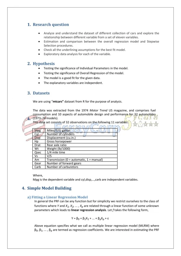
1.Research question Analyze and understand the dataset of different collection of cars and explore the relationship between different variable from a set of eleven variables. Estimation and comparison between the overall regression model and Stepwise Selection procedures. Check all the underlining assumptions for the best fit model. Exploratory data analysis for each of the variable. 2.Hypothesis Testing the significance of Individual Parameters in the model. Testing the significance of Overall Regression of the model. The model is a good fit for the given data. The explanatory variables are independent. 3.Datasets We are using “mtcars” dataset from R for the purpose of analysis. The data was extracted from the 1974 Motor Trend US magazine, and comprises fuel consumption and 10 aspects of automobile design and performance for 32 automobiles (1973–74 models). 4. This data set consists of 32 observations on the following 11 variables: Mpg Miles/(US) gallon Cyl Number of cylinders Disp Displacement (cu.in.) Hp Gross horsepower Drat Rear axle ratio Wt Weight (lb/1000) Qsec 1/4 mile time Vs V/S Am Transmission (0 = automatic, 1 = manual) Gear Number of forward gears Carb Number of carburetors Where, Mpg is the dependent variable and cyl,disp,…,carb are independent variables. 4. Simple Model Building a) Fitting a Linear Regression Model In general the PRF can be any function but for simplicity we restrict ourselves to the class of functions where Y and X1, X2, ... , Xp are related through a linear function of some unknown parameters which leads to linear regression analysis. Let f takes the following form, Y = β0+ β1X1+ ... + βpXp+ ε Above equation specifies what we call as multiple linear regression model (MLRM) where β0, β1, ... , βp are termed as regression coefficients. We are interested in estimating the PRF
which is equivalent to estimate the unknown parameters β0, β1, ... , βp on the basis of a random sample from Y and given values of the independent variables. Here, we take in our study, “mpg” as dependent variable an rest all other variables viz. “cyl”, “disp”, “hp”, etc. as independent variables X1, X2, ... , Xp. “mpg” = β0+ β1“cyl” + ... + βp“carb” + ε Coefficients 12.303 -0.111 0.013 -0.021 0.787 -3.715 0.821 0.318 2.520 0.655 -0.199 Standard Error 18.718 1.045 0.018 0.022 1.635 1.894 0.731 2.105 2.057 1.493 0.829 t Stat 0.657 -0.107 0.747 -0.987 0.481 -1.961 1.123 0.151 1.225 0.439 -0.241 P-value 0.518 0.916 0.463 0.335 0.635 0.063 0.274 0.881 0.234 0.665 0.812 Intercept Cyl Disp Hp Drat Wt Qsec Vs Am Gear Carb In the above table regression coefficients β0, β1, ... , βp are represented by column “coefficients”. This means, with a unit change in the explanatory variable, there is a coefficient times change in the dependent variable. Ex. With 1 unit change in the velocity (vs) there is a 0.318 unit change in the dependent variable (mpg). After estimating the unknown parameters involved in a multiple linear regression model, the next task of interest is to test for their statistical significance. b) Testing the significance of Individual Parameters Under normality assumption for the error terms, significance of individual parameters can be tested using a t-test. The procedure is as follows: Step 1: Null Hypothesis is set as H0:βi= 0 and Alternative Hypothesis is set as H1:βi≠0. Step 2: Calculate the t-statistic as follows: Step 3: Reject H0if p value of calculated t statistic is less thanα= 0.05 and conclude thatthe βi is statistically significant at 5% l.o.s. otherwise accept H0. For the model under study, we have- refer the above table. Conclusion From the above table, since p-value of all the parameters are greater than 0.05, hence we may conclude that all the individual parameters are insignificant at 5% l.o.s. Only “wt” is significant at 10% l.o.s.
c) Testing the significance of Overall Regression Under normality assumption for the error terms, significance overall regression can be tested using an F-test. The procedure is as follows: Step 1: Null hypotheses is H0:β1= β2=…=βp= 0 and Alternative hypothesis is H1:βi≠0 forat least one i = 1, 2, ... , p. Step 2: Calculate the F-statistic as follows: where MS Reg and MS Res are the mean sum of squares due to regression and residuals. Step 3: Reject H0if p value of calculated F statistic is less than α= 0.05 i.e. the overall regression is statistically significant. For the model under study, we have ANOVA Df 10 21 31 SS MS 97.855 7.024 F Significance F 0.000 Regression Residual Total 978.553 147.494 1126.047 13.933 Conclusion From the above table, since p-value is less than 0.05, hence we may conclude that the overall regression is significant at 5% l.o.s. d) R Square and Adjusted R Square R-Square, also termed as coefficient of determination is a measure of goodness of model. It is defined as follows: R2represents the proportion of variability explained by the model. Clearly 0 ≤ R2≤ 1. An adequate model is expected to have high R2. It can be proved that R2 is an increasing function of the number of independent variables included in the model and hence it doesn’t give true insight about goodness of the model. A refined measure of goodness which is free from this drawback, termed as adjusted R2 is defined as follows. It can be observed that - ∞ ≤ R2 adj ≤ R2≤ 1 . For the model under study, we have
Regression Statistics Multiple R R Square Adjusted R Square Standard Error Observations 0.932 0.869 0.807 2.650 32 Conclusion From the above table, since R2 is a good fit for the given data. From the above hypothesis testing we see a high value of overall R2 but insignificant t-ratios indicating that Multicollinearity may be present among the independent variables. adj is quite high, hence we may conclude that the selected model 4.1Multicollinearity a)Problem and its Consequences The existence of near linear relationship among the explanatory variables is termed as Multicollinearity. In other words multicollinearity is a situation when one or moreexplanatory variables can be well expressed as a near linear combination of the other explanatory variables. Multicollinearity can arise due to several reasons like use of too many regressors, faulty data collection etc. In has been seen that presence of multicollinearity seriously weakens the results based on ordinary least squared technique. Following are the common ill consequences of this problem: 1.Variances of the ordinary least squares estimates of the regression coefficients are inflated. 2.Absolute values of the regression coefficients are very high. 3.Regressors which are expected to be important turn out to be insignificant. 4.Regressors have wrong sign as against the a priori belief. b)Detection and Removal of Multicollinearity Variance Inflation Factor (VIF) Approach: Define R2 (j) = R2 of the multiple linear regression model where Xj is taken as dependent variable and all other regressors X1, ... , Xj-1 , Xj+1 , ... , Xp . Clearly R2 (j) is expected to be high if there is a strong linear relationship between Xj and the rest of the regressors. It can be shown that Variance Inflation Factor (VIF) of the jth regressor defined as follows. Clearly R2 (j) and VIFj are positively related and hence VIFj is expected be high if jth is involved in
multicollinearity. Detection: As a rule-of-thumb if VIFj> 10 then Xjcan be taken to have strong linear relationship with the other regressors. Removal: Deleting the corresponding Xj‘s will solve the problem. For the model under study, we have Model VIF Cyl 15.374 Disp 21.62 Hp 9.832 Drat 3.375 Wt 15.165 Qsec 7.528 Vs 4.966 Am 4.648 Gear 5.357 Carb 7.909 Conclusion We see that the highlighted variables are significant (i.e., VIFi > 10 ). Thus, to counter the problem of multicollinearity we remove “cyl”, “disp” and “wt”. For the reduced model, we get, Regression Statistics Multiple R R Square Adjusted R Square Standard Error Observations 0.914 0.836 0.788 2.775 32 From the above approach used for the removal of multicollinearity, we find that Variance Inflation Factor (VIF) approach is a good fit to the given data. 5. Analysis of single data set. For visualization, we are now categorizing the data set into continuous and categorical variables. In the given data set we have the following continuous variables: 1.mpg – Miles/(US) gallon 2.disp – Displacement 3.hp – Gross Horsepower 4.drat – Rear axle ratio 5.wt – Weight (lb/1000) 6.qsec – ¼ mile time.
We are using the following measures/ tools for visualization: 1.Q-Q PLOTS: To test whether the data is normally distributed or not with the hypothesis: Ho: Sample comes from a normal population. H1: Sample does not come from the normal population. 2.BOX-PLOTS: To determine if there are any outliers in the data. 3.DESCRIPTIVE STATISTICS: Like mean, median, mode, etc. MPG :- Miles/(US) gallon: QQ-PLOT (mpg) Statistical moments OBSERVED VALUES 40 Values 30 μ1 20.09 20 10 μ2 36.32 0 μ3 -498495 -3.000 -2.000 -1.000 0.000 1.000 2.000 3.000 μ4 15262466 EXPECTED VALUES BOX-PLOT (mpg) 5.00 10.00 15.00 20.00 25.00 30.00 From the normal QQ-Plots we may infer that “mpg” is almost normally distributed. From Box-Plots we may infer that “mpg” does not contain any outlier. 2)DISP-Displacement: Statistical moments μ1 μ2 μ3 μ4 Values 230.7219 15360.8 -7.4E+08 2.77E+11
QQ-PLOT(disp) 600 OBSERVED VALUES 400 200 0 -3.000 -2.000 -1.000 0.000 1.000 2.000 3.000 -200 EXPECTED NORMAL BOX-PLOT (disp) 0.00 100.00 200.00 300.00 400.00 500.00 From the QQ-Plot we may infer that “disp” is not normally distributed. From the box plots we may infer that “disp” does not contain any outlier. 3)HP-GROSS HORSE POWER: QQ-PLOT(hp) Statistical moments Values μ1 μ2 μ3 μ4 400 OBSERVED VALUES 146.6875 4700.867 -1.9E+08 4.51E+10 300 200 100 0 -4.000 -2.000 0.000 2.000 4.000 EXPECTED NORMAL
BOX-PLOT (hp) 31 0.00 100.00 200.00 300.00 400.00 From the above QQ-Plots we may infer that “hp” is not normally distributed. From the box plots we may infer that “hp” contains an outlier as 31st observation. 4)DRAT-Rear axle ratio: QQ-PLOT(drat) Statistical moments Values 6 μ1 3.596563 5 OBSERVED VALUES 4 μ2 0.285881 3 μ3 -2883.09 2 μ4 15566.83 1 0 -3.000 -2.000 -1.000 0.000 1.000 2.000 3.000 EXPECTED NORMAL BOX-PLOT (drat) 0.00 1.00 2.00 3.00 4.00 5.00 6.00 From the above QQ-Plot we may infer that “drat” may be almost normally distributed.
From the box plot we may infer that “drat” does not contain any outlier. 5)WT-weight(lb/1000) Statistical moments QQ-PLOT(wt) values 6 μ1 3.21725 OBSERVED VALUES 4 μ2 0.957379 2 μ3 -2051.96 0 μ4 10051.06 -4.000 -2.000 0.000 2.000 4.000 EXPECTED NORMAL BOX-PLOT (wt) 16 17 0.00 1.00 2.00 3.00 4.00 5.00 6.00 From the QQ-Plot we may infer that “wt” is almost normally distributed. From box plot we may infer that “wt” has 2 outliers which are 16th and 17th observations. 6)QSEC-1/4 mile time Statistical moments μ1 μ2 μ3 μ4 Values 17.84875 3.193166 -352478 9439831
QQ-PLOT(qsec) 25 OBSERVED VALUES 20 15 10 5 0 -3.000 -2.000 -1.000 0.000 1.000 2.000 3.000 EXPECTED NORMAL BOX-PLOT (qsec) 9 10.00 15.00 20.00 25.00 30.00 From the QQ-Plot we may infer that “qsec” is almost normally distributed. From the box plot we may infer that “qsec” contains an outlier as 9th observation. 2. In the given data set we have the following discrete variables: 1.cyl – Number of cylinders 2.vs – V/S 3.am – Transmission (0=automatic, 1=manual) 4.gear – Number of forward gears 5.carb – Number of carburetors We will use the following measures/tools: 1.Frequency Table To get the frequency of each data point. 2.Bar Plot To represent the frequency distribution of data. 1)CYL-no of cylinders Frequency table:
valid 4 6 8 total Bar Graph: Frequency 11 7 14 32 Cumulative percent 34.4 56.2 100 16 14 statistical moments 12 10 μ1 6.187 8 6 μ2 3.189 4 2 μ3 -147 0 number of cyl=4 number of cyl=6 number of cyl=8 μ4 136 2)VS-V/S Frequency Table: Valid 0 1 Total Bar graph: Frequency 18 14 32 Cumulative Frequency 56.2 100 20 18 16 statistical moments 14 12 μ1 0.4375 10 8 μ2 0.254032 6 4 μ3 -4.20752 2 0 μ4 5.468216 vs=0 vs=1 3)AM-TRANSMISSION (0=automatic, 1=manual) Frequency table: valid Frequency 0 19 1 13 total 32 Cumulative Frequency 59.4 100
Bar graph: 20 statistical moments 15 μ1 0.40625 10 μ2 0.248992 5 μ3 -2.70966 0 μ4 4.666333 automatic manual 4)GEAR-Number of forward gears: Frequency table: Valid 3 4 5 Total Bar graph: Frequency 15 12 7 32 Cumulative percentage 46.9 84.4 100 16 statistical moments 14 μ1 3.6875 12 10 μ2 0.544355 8 6 μ3 -3101.97 4 2 μ4 17213.65 0 fwd gear=3 fwd gear=4 fwd geaR=5 5)CARB- number of carburetors: Frequency table: Valid One Two Frequency 7 10 Cumulative percentage 21.9 53.1
Three Four Six Eight Total Bar graph: 3 10 1 1 32 62.5 93.8 96.9 100 12 10 statistical moments 8 μ1 2.8125 6 μ2 2.608871 4 μ3 -1237.63 2 0 One Two Three Four Six Eight 6. Correlations Y and every x data set: correlation of y (mpg) with : Cyl Disp Hp Drat Wt Qsec Vs Am Gear Carb All combinations of x data sets: Values -0.852 -0.848 -0.776 0.681 -0.868 0.419 0.664 0.599 0.480 -0.551 x on x Cyl disp Hp drat wt Qsec vs am Gear carb Cyl 1 0.902 0.832 -0.700 0.782 -0.591 -0.811 -0.523 -0.493 0.527 Disp 0.902 1 0.791 -0.710 0.888 -0.434 -0.710 -0.591 -0.556 0.395 Hp 0.832 0.791 1 -0.449 0.659 -0.708 -0.723 -0.243 -0.126 0.750
Drat -0.700 -0.710 -0.449 1 -0.712 0.091 0.440 0.713 0.700 -0.091 Wt 0.782 0.888 0.659 -0.712 1 -0.175 -0.555 -0.692 -0.583 0.428 Qsec -0.591 -0.434 -0.708 0.091 -0.175 1 0.745 -0.230 -0.213 -0.656 Vs -0.811 -0.710 -0.723 0.440 -0.555 0.745 1 0.168 0.206 -0.570 Am -0.523 -0.591 -0.243 0.713 -0.692 -0.230 0.168 1 0.794 0.058 Gear -0.493 -0.556 -0.126 0.700 -0.583 -0.213 0.206 0.794 1 0.274 Carb 0.527 0.395 0.750 -0.091 0.428 -0.656 -0.570 0.058 0.274 1 We know, Correlation coefficient measures the degree of linear relationship between two variables. Possible two variable linear relationships between regressors can be detected if some pair wise correlations are significant. Consider the matrix of all pair wise correlations. As a rule-of-thumb if |rij|> 0.5 then Xiand Xjcan be taken to have strong linearrelationship. We see that the highlighted correlations are significant (i.e., | rij | > 0.5). Here we can note that the correlation matrix also resolves the problem of multicollinearity. Thus, to counter the problem of multicollinearity we can remove “disp”, “hp”, “wt”, “cyl”, “vs” and “am”. 7. Regression Y for different selections of X A parsimonious model is a model that accomplishes a desired level of explanation or prediction with as few predictor variables as possible. To achieve such type of model, we are here using the technique of stepwise selection. Stepwise selection is a method that allows moving in either direction, dropping (backward elimination) or adding(forward selection)variables at the various steps. The process is one of alternation between choosing the least significant variable to drop and then re-considering all dropped variables (except the most recently dropped) for re-introduction into the model. For the given data, we run stepwise regression, following results can be obtained: ANOVA (predictors:wt,cyl) Regression 2 Df SS 934.875 MS 467.438 F 70.908 Significance F 0.000 191.172 6.592 Residual 29 1126.047 Total 31 Regression Statistics Multiple R R Square Adjusted R Square Standard Error Observations 0.911 0.830 0.819 2.568 32 Conclusion Thus the model selected by stepwise selection method is: “mpg” = β0+ β1“wt” + β2“cyl” + ε
From parsimonious modeling, we find that model selected by stepwise selection model has less predictors making the model more parsimonious. Hence, we will consider the model i.e., “mpg” = β0+ β1“wt” + β2“cyl” + ε 8. Validation of Assumptions and Residual Analysis There are four principal assumptions which justify the use of linear regression models for purposes of inference or prediction: a)linearity and additivity of the relationship between dependent and independent variables. b)statistical independence of the errors (in particular, no correlation between consecutive errors in the case of time series data) c)homoscedasticity (constant variance) of the errors d)normality of the error distribution. a)Linearity of Regression In Classical Multiple Linear Regression Model we assume that the relationship between y and X1, ... , Xp is linear in terms of both parameters and independent variables. We are interested in validating the linearity in terms of independent variables. Linearity of individual regressors in the complete model can be validated using the partial regression plots. For the model under study, we have partial regression plots as: From the partial regression plot of mpg on cyl we may refer that mpg and cyl are almost linearly related From the partial regression plot of mpg on wt we may refer that mpg and wt are almost linearly related
b)Autocorrelation When error terms for different sample observations are correlated to each other, i.e. there is a linear relationship among the error terms the situation is called as autocorrelation or serial correlation. We are interested in detecting if there is an autocorrelation present in the model. This can be done using the Durbin-Watson Test. Durbin Watson Test is based on the assumption that the errors in regression model are generated by a first order autoregressive (AR(1)) process that is, εi= ρεi-1+ δi 2) and |ρ| < 1 is the autocorrelation parameter. where δi~iid N(0,σδ We set up the hypotheses as follows: Null Hypothesis Alternative Hypothesis H1: ρ ≠ 0 Presence of Autocorrelation Durbin Watson test statistic is given by, HO:ρ = 0 Absence of Autocorrelation It can be seen that D ≈ 2(1-r) where r is the sample autocorrelation coefficient of the residuals and 0 ≤ D ≤ 4. Hence D = 2 means no autocorrelation. Thus, we have Durbin watson statistic: 1.617 Conclusion Thus we have Durbin-Watson statistic D = 1.671 ≈ 2. Hence we may conclude that the model selected by stepwise selection method does not have autocorrelation. c)Heteroscedasticity When error terms for different sample observations have same variances the situation is called as homoscedasticity. opposite of homoscedasticity is called as hetroscedasticity. We are interested in detecting if there is a hetroscedasticity present in the model. We can do this by plotting the predicted dependent variables with the square of the residuals. Since the 7.000 6.000 The 5.000 4.000 3.000 2.000 1.000 0.000 0.000 5.000 10.000 15.000 20.000 25.000 30.000 35.000 points do not show any specific pattern, so, from the above scatter plot we may infer that model is homoscedastic. In other words there is no hetroscedasticity in the model. d)Normality of Errors
We can test the normality of error by means of plotting quantiles of the standardized resiudals against those of a standard normal distribution. Expected Normal Values Normal QQ-Plot 3.000 2.000 1.000 0.000 -3 -2 -1 0 1 2 3 -1.000 -2.000 -3.000 Observed Values From the normal Q-Q Plot, it can be observed that most of the observations lie around the straight line but few deviate from the line. Thus, we may conclude that the Residuals are almost normally distributed with 0 mean and variance σ². 9. Analysis of the results The tables below represent the regression statistics for the model when all the variables are taken into consideration and the reduced model (stepwise selection). Regression Statistics(overall) Multiple R R Square Adjusted R Square Standard Error Observations Regression Statistics(reduced) Multiple R R Square Adjusted R Square Standard Error 0.932 0.869 0.807 2.650 32 0.911 0.830 0.819 2.568 Observations 32 We can clearly observe that the reduced model is a better fit to the given data as it has a higher adjusted R2 and involves less number of variables making the model less complex and easy to understand. Moreover, the reduced model not only overcomes the problem of multicollinearity but also validates all the underlining assumptions of regression (refer pt 8).
Sources: Source of Data -Henderson and Velleman (1981), Building multiple regression models interactively. Biometrics, 37, 391–411. Books -Gupta and Kapoor, Fundamentals Of Mathematical Statistics, Sultan Chand and Sons, 1970. -John W. Tukey., Exploratory Data Analysis, Addison-Wesley, 1977. -Gupta and Kapoor, Fundamentals Of Applied Statistics, Sultan Chand and Sons, 1970. -Chatterjee, S. and Price, B. Regression Analysis by Example. Wiley, New York, 1977. -Darius Singpurwalla, A Handbook Of Statistics, An overview of statistical methods, 2013. -Mosteller, F., & Tukey, J. W. Data analysis and regression: A second course in statistics. Reading, MA: Addison-Wesley, 1977. World Wide Web -https://flowingdata.com/2008/02/15/how-to-use-a-box-and-whisker- plot/ -http://www.law.uchicago.edu/files/files/20.Sykes_.Regression.pdf -http://www.123helpme.com/search.asp?text=regression+analysis -https://www.youtube.com/watch?v=eYp9QvlDzJA.