Scattered data fitting using least squares with interpolation method
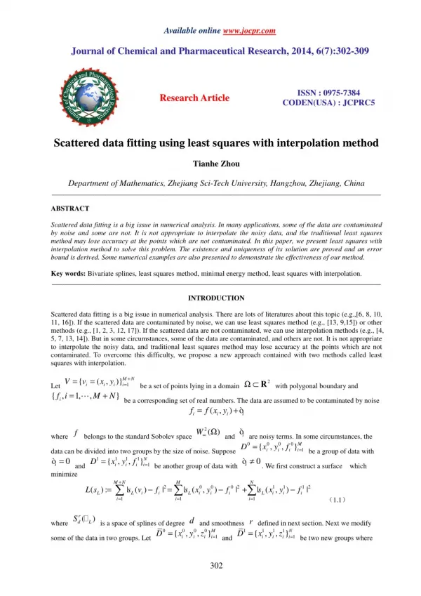
Scattered data fitting is a big issue in numerical analysis. In many applications, some of the data are contaminated<br>by noise and some are not. It is not appropriate to interpolate the noisy data, and the traditional least squares<br>method may lose accuracy at the points which are not contaminated. In this paper, we present least squares with<br>interpolation method to solve this problem. The existence and uniqueness of its solution are proved and an error<br>bound is derived. Some numerical examples are also presented to demonstrate the effectiveness of our method.

Scattered data fitting using least squares with interpolation method
E N D
Presentation Transcript
Available online www.jocpr.com Journal of Chemical and Pharmaceutical Research, 2014, 6(7):302-309 ISSN : 0975-7384 CODEN(USA) : JCPRC5 Research Article Scattered data fitting using least squares with interpolation method Tianhe Zhou Department of Mathematics, Zhejiang Sci-Tech University, Hangzhou, Zhejiang, China _____________________________________________________________________________________________ ABSTRACT Scattered data fitting is a big issue in numerical analysis. In many applications, some of the data are contaminated by noise and some are not. It is not appropriate to interpolate the noisy data, and the traditional least squares method may lose accuracy at the points which are not contaminated. In this paper, we present least squares with interpolation method to solve this problem. The existence and uniqueness of its solution are proved and an error bound is derived. Some numerical examples are also presented to demonstrate the effectiveness of our method. Key words:Bivariate splines, least squares method, minimal energy method, least squares with interpolation. _____________________________________________________________________________________________ INTRODUCTION Scattered data fitting is a big issue in numerical analysis. There are lots of literatures about this topic (e.g.,[6, 8, 10, 11, 16]). If the scattered data are contaminated by noise, we can use least squares method (e.g., [13, 9,15]) or other methods (e.g., [1, 2, 3, 12, 17]). If the scattered data are not contaminated, we can use interpolation methods (e.g., [4, 5, 7, 13, 14]). But in some circumstances, some of the data are contaminated, and others are not. It is not appropriate to interpolate the noisy data, and traditional least squares method may lose accuracy at the points which are not contaminated. To overcome this difficulty, we propose a new approach contained with two methods called least squares with interpolation. { ( , )}M N i i i i V v x y = = = be a set of points lying in a domain { , 1, , } M N = + L be a corresponding set of real numbers. The data are assumed to be contaminated by noise ( , i i f f x y = where f belongs to the standard Sobolev space + Ω ⊂ R with polygonal boundary and 2 1 Let if i +ò ) i i W∞Ω and 2( ) iò are noisy terms. In some circumstances, the 0 0 0 0 1 { , , }M i i i i D x y f = = be a group of data with 0 ò . We first construct a surface which data can be divided into two groups by the size of noise. Suppose 0 ò and minimize M N L s s v = i= i≠ = 1 1 i 1 i 1 }N i { , x y , D f = 1 be another group of data with i + M N ∑ ∑ ∑ = − = − + − 2 0 i 0 i 0 2 1 i 1 i 1 2 ( ): L | ( ) L | | ( L s x , ) | | ( , L s x y ) | f y f f i i i i = = (1.1) 1 1 1 i i i r d ( ) S is a space of splines of degree d and smoothness r defined in next section. Next we modify 0 0 0 0 1 { , , }M i i i i D x y z = = and L where = 1 1 i 1 i 1 i , }N { , x y z D = 1 i some of the data in two groups. Let be two new groups where 302
Tianhe Zhou J. Chem. Pharm. Res., 2014, 6(7):302-309 ______________________________________________________________________________ = − iz = 0 i 0 0 i 0 i 1: 0 r d : ( , ) ( ) z f s x y S and . Define a set of all spline in that interpolate the data at the points i L I of V by : { = ∈ = = = … = … 0 i 0 i 0 i 1 j 1 j 1 j r d ( ): ( I , ) , ( , z s x y ) , 1, , , 1, , }. N I s S s x y z i M j f (1.2) ∈ r d ( ) s S I is a new triangulation of data locations. After that, we construct a spline function where that such I I = ∈ ( ) E s min{ ( ): E s } s I I f (1.3) ( ) E s is a energy function defined by where =∑∫ + + 2 xx 2 xy 2 y ( ): s [ 2 ]. E s s s y T ∈∆ T I Finally, we get a new spline function by = + . s s s F L I (1.4) Ls L From the above, we can see that it need to construct two splines with two triangulations in our approach. One is Is for data interpolation. We construct the spline Is base on In this paper, we derive the following error bound for this approach, 2 , 1 2 (2 | | | | )| F L f s C C ∞ Ω − ≤ + ‖ ‖ Ls base on triangulation for least squares fit, another one is I. and the 2 2, , | , f ∞ Ω I (1.5) | | f f ‖‖ ∞ Ω denotes the maximum norm of the second order derivatives of f over Ω and L ∞ Ω 2, , , where standard infinity norm of f over Ω. Here | | L and The paper is organized as follows. In Section 2 we review some well-known Bernstein-Bezier notation. The result on error bounds of this approach is derived in Section 3 together with a discussion on existence and uniqueness. In Section 4 we present some numerical examples for our method. PRELIMINARIES Given a triangulation and integers 0 r d , we write ( ): { ( ): | d S s C = ∈ Ω is the and | | I are the maximum of the diameters of the triangles in I and all the constants in the error bound will be introduced in following sections. ≤ < ∈ ∈ r r ,for all } s P T T d d + dimensional space of 2 dP is the 2 for the usual space of splines of degree d and smoothness r, where bivariate polynomials of degree d. Throughout the paper we shall make extensive use of the well-known = 〈 〉 in with vertices , , , , , T v v v v v v 1 2 3 1 2 3 Bernstein-Bezier representation of splines. For each triangle the |T s corresponding polynomial piece is written in the form = ∑ T ijk T ijk | , s c B T j k d + + = i T ijk ( , λ λ λ B , ) are the Bernstein-Bezier polynomials of degree d associated with T. In particular, if 1 2 3 where 303
Tianhe Zhou J. Chem. Pharm. Res., 2014, 6(7):302-309 ______________________________________________________________________________ u∈R relative to the triangle T, then 2 are the barycentric coordinates of any point ! d = λ λ λ + + = T ijk i j k ( ): u , . B i j k d 1 2 3 ! ! ! i j k c T ijk i j k d + + = with the domain points As usual, we associate the Bernstein-Bezier coefficients { { : ( )/ } ijk iv jv kv d ξ = + + Definition 1. Let β < ∞. A triangulation is said to be β-quasi-uniform provided that | | ρ is the minimum of the radii of the incircles of triangles of . We say the data locations are evenly distributed over each triangle of , if there are enough data points for every triangle such that ( T P C ∞ ≤ ‖ ‖ } T . i j k d + + = 1 2 3 ≤ βρ , where ∑ 2 1/2 ( ) ) i P v , v T ∈ i for any polynomial P and some constant C. ERROR ANALYSIS In this section, we mainly discuss the error bounds for the spline function created by this approach. First, we show Ls is a solution of least squares method and of minimal energy interpolation. Is is a solution the existence and uniqueness of this spline. Note that L . Then there Theorem 3.1 (cf. [15] ) Suppose all the data locations are evenly distributed over each triangle of ( ) L d L s S ∈ satisfying (1.1). r exists a unique ∈ r d ( ) s S Theorem 3.2 (cf. [7] ) There exists a unique solution s s s = + , we can get which satisfies (1.3). I I F L I Note that Fs Theorem 3.3 There exists a unique solution Next we show the error bound for the spline function. Recall from [10], we can get f s C ∞ Ω − ≤ ‖ ‖ of this approach. 2 | | | L 2, , | . f ∞ Ω , 1 L (3.1) ∈ 2( ) Ω. Then there f W∞ I are β-quasi-uniform and L and Theorem 3.4 Suppose that two triangulations C and Fs defined in (1.4) satisfies (2 | F f s C ∞ Ω − ≤ ‖ ‖ C depending on d, β, Cand the smallest angel in each triangulation such 1 2 exists two constants that the spline + 2 L 2 | | )| I 2, , | . C f ∞ Ω , 1 2 = + s s s Proof: Since F L I , we can get 304
Tianhe Zhou J. Chem. Pharm. Res., 2014, 6(7):302-309 ______________________________________________________________________________ − = − − ≤ − + ‖ ‖ ,. ∞ Ω f s f s s f s s ‖ F ‖ ‖ I ‖ ‖ L ‖ ∞ Ω ∞ Ω ∞ Ω , , , L I (3.2) Is is a minimal energy spline that interpolate the data 2( ) z W∞ ∈ Ω. Recall from [11], we can get 0 1 D and D. We can assume that the data Note that comes from a function − ≤ 2 | | | I 2, , | . s z ‖ C f ‖ ∞ Ω ∞ Ω , 2 I (3.3) = − iz = f ‖ 0 i 0 0 i 0 i z 1: 0 − : ( , ) z f s x y Since and , we have ,. ∞ Ω ‖ i L ≤ s ‖‖ ∞ Ω , L (3.4) Then by (3.3) and (3.4), we have s ∞ Ω ‖ ‖ = − + ≤ − + ‖‖ ≤ + ‖ − 2 | | | I 2, , | . s z z ‖ s z ‖ z C f f s ‖ ‖ L ‖ ∞ Ω ∞ Ω ∞ Ω ∞ Ω ∞ Ω , , , , 2 , I I I (3.5) Therefore, by substituting (3.1) and (3.5) into (3.2), we have − ≤ + 2 2 (2 | | | | )| I 2, , | . f s C C f ‖ F ‖ ∞ Ω ∞ Ω , 1 2 L This completes the proof. NUMERICAL EXAMPLE In this section, we present a numerical example to demonstrate the performance of our approach. 0 0 0 0 0 {( , , ( , ))} i i i i D x y f x y = {( , , ( , ) i i i i D x y f x y = +ò be a scattered data setwhich is marked with a triangle without )} be a contaminatedscattered data set which is marked with a f x y is a test function and the following test functions 4 4 1( , ) 2 , 5 f x y x y = + 2( , ) sin(2( )), f x y x y = − 3( , ) 0.75exp( 0.25(9 f x y = − 0.75exp( (9 x + − + 0.5exp( 0.25(9 + − 0.2exp( (9 x − − − Example 4.1 Let 1 1 1 1 1 contaminated and iò is a random number between 0.01 − ( , ) to 0.01. We use circle in Fig. 1, where − − − 2 2 2) 0.25(9 y + 0.25(9 7) ) y − 2) ) x y − 2 1) /49 (9 7) x − 2 4) (9 − 1)/10) y − − 2 2 3) ) 2 . 1 5( Ls, where I as 1 1 , }N i i x y z ) S to evaluate the scattered data set. First we use the spline space L is the triangulation given in Fig. 1. Next we triangulate all data locations to get a new triangulation to find the the fitting surfaces L = = 0 0 i 0 i 0 i 1 1 i }M i { , , { , D x y z D = = 1 1 shown in Fig. 2. We modify some of the data in two groups. Let 0 : i z s S ∈ maximum errors against the exact function between our approach the traditional least squares method and weighted and i = − iz = 0 i 0 i 0 i 0 i 1: 0 ( , ) ( , ) f x y s x y be two new groups where and . Then we construct a minimal energy s s = + . Moreover, we compared the L 1 5( ) s F L I interpolatory spline . Finally, we can get our solution by I I 305
Tianhe Zhou J. Chem. Pharm. Res., 2014, 6(7):302-309 ______________________________________________________________________________ i ω = 1 least squares method (cf. [15]) in Table 1. Here in weighted least squares method, the weights are set to be 0.01 for the exact data and contaminated data, respectively. The maximum errors are measured using 101 101 × × . Table 1: Approximation errors. Test functions Our method Traditional l.s. method 1( , ) f x y 0.0342 0.4383 2( , ) f x y 0.0474 0.4778 3( , ) f x y 0.0441 0.2988 Discussion: From Table 1, we can see that the error bounds of our approach is better than that of the traditional least squares method. And compare to weighted least squares method, it is hard to say which method is better. But there is a one big difference between our method and weighted least squares method. That is the surface created by our method can pass through the exact data. i ω = and equally-spaced points over [0,1] [0,1] Weighted l.s. method 0.0965 0.0407 0.0216 L Figure 1. Scattered data and triangulation Below, we present an example to illustrate an application of our method. Example 4.2 We consider the shape design of a car. For example, the hood (a part of a car). A set of data are given in Fig. 3 which are used to construct the hood. The data can be divided into two groups. One is marked with triangle which means the shape must go through the data (For instance, the edge of the hood). That means we need to interpolate these data. The other is marked with cycle which need to be least squares fit. We first use the spline space 1 5( ) L S to find the the fitting surfaces Ls, where L is the triangulation given in Fig. 3. Next we modify two ∈ 1 5( ) s s S I groups of data from our method, then we construct a minimal energy interpolatory spline , where s + I I = s F L I is a new triangulation of all data locations given in Fig. 4. Finally, we draw the shape of the hood shown in Fig. 5. as 306
Tianhe Zhou J. Chem. Pharm. Res., 2014, 6(7):302-309 ______________________________________________________________________________ I Figure 2. Triangulation of data locations L Figure 3. Data locations and triangulation 307
Tianhe Zhou J. Chem. Pharm. Res., 2014, 6(7):302-309 ______________________________________________________________________________ I Figure 4. Triangulation of data locations Figure 5. The shape of the hood Acknowledgments This work is supported by National Natural Science Foundation of China under Grant No.11201429. 308
Tianhe Zhou J. Chem. Pharm. Res., 2014, 6(7):302-309 ______________________________________________________________________________ REFERENCES [1]D. L. Ragozin. J. Approx. Theory. v33, pp.335-355, 1983. [2]M. C. Lopez de Silanes, R. Arcangeli,.Sur la convergence des Dm--splines d'ajustement pour des données exactes ou bruitées, Revista Matemática de la Universidad Complutence de Madrid. v4, pp 279-284, 1991. [3]R.Arcangeli, B.Ycart, Almost sure convergence of smoothing Dm-spline functions. Numer. Math. v66, pp.281-294, 1993. [4]M. J. Lai. Comput. Aided Geom. Design. v. 13, pp. 81-88, 1996. [5]M. J. Lai, L. L. Schumaker, SIAM J. Numer. Anal. v.34, pp.905-921, 1997. [6]M. J. Lai, L. L. Schumaker, On the approximation power of bivariate splines, Adv. in Comp. Math. v.9, pp251-279, 1998. [7]K. Farmer, M. J. Lai. Scattered data interpolation by C2 quintic splines using energy minimization, Approximation Theory IX, pp. 47-54, 1998. [8]O. Davydov,L. L. Schumaker, On stable local bases for bivariate polynomial spline spaces, Constr. Approx. v 18, pp 87-116, 2001. [9]M. von Golitschek, L. L. Schumaker,. Bounds on projections onto bivariate polynomial spline spaces with stable local bases, Constr. Approx, v.18, pp 241-254, 2002. [10]M. von Golitschek, M. J. Lai, L. L. Schumaker, , Numer. Math, pp.315-331, 2002. [11]R. Arcangeli, M. C. Lopez de Silanes, J. J. Torrens, Multidimensional minimizing splines, Kluwer Academic Publishers,2004. [12]G. Awanou, M. J. Lai, P. Wenston, Wavelets and Splines, pp 24-74, 2006. [13]T. Zhou, D. Han, M. J. Lai Appl. Numer. Math. v 58, pp 646-659, 2008. [14]T. Zhou, D. Han. J. Comput. Appl. Math. v 217, pp 56-63, 2008. [15]M. J. Lai, L. L. Schumaker, Spline Functions on Triangulations, United Kingdom at the University Press, Cambridge.2007. [16]A. Kouibia, M. Pasadas. J. Comput. Appl. Math. v 211, pp 213-222, 2008. 309