Modeling laminar flow between infinite parallel plates using the SIMPLE algorithm
Overview. Motivation Problem StatementAnalytical SolutionNumerical ProcedureResults Conclusion. Motivation. CFD is an integral part of design and analysisHow does commercial CFD code work ? or perhaps how do we get these cool pictures ?. Problem Statement. Calculate the velocity profile in a fully developed laminar flow between infinite parallel platesModel flow between the annular gap between a piston and cylinder (calculate leakage flow rate).

Modeling laminar flow between infinite parallel plates using the SIMPLE algorithm
E N D
Presentation Transcript
1. Modeling laminar flow between infinite parallel plates using the SIMPLE algorithm Gopi Krishnan
12/09/2004
3. Motivation CFD is an integral part of design and analysis
How does commercial CFD code work ? or perhaps how do we get these cool pictures ?
4. Problem Statement Calculate the velocity profile in a fully developed laminar flow between infinite parallel plates
Model flow between the annular gap between a piston and cylinder (calculate leakage flow rate)
5. Analytical Solution
6. Analytical Solution Assumptions
Steady flow
Incompressible
Fully developed flow
Infinite in z direction
No body forces
7. Numerical Approach Pressure Correction technique
Wide-spread application for numerical solution of incompressible N-S equations
SIMPLE ( Semi-Implicit Method for Pressure Linked equation) Patankar and Spalding, 1972
8. Pressure Correction Staggered grid
Velocity and Pressure are calculated at different grid points
9. Pressure Correction Method Guess a pressure field; p*
Solve for velocities from momentum equation; u*,v*
Since u*, v* are guessed vales they will not satisfy the continuity equation. So construct a pressure correction p` to get the velocity to agree with continuity;
p = p* + p`
Solve for velocities using new pressure
Repeat till velocities satisfy continuity equation
10. Pressure Correction Forward difference in time
Central difference in spatial derivatives
p` ; Creating a numerical artifice to get u, v to satisfy continuity
Construct the difference equation for the x and y momentum equations for guessed variables (u*,v*,p*) and updated variables (u,v,p)
Algebraic manipulation to get u`n+1, v`n+1 in terms of u`n, v`n, p`n
Pressure correction formula; p`
11. Pressure Correction Central assumption ; (ru`)n and (rv`)n = 0
Other schemes make different approximations
ap�i,j + bp�i+1,j + bp`i-1,j + cp`i,j+1 + cp`i,j-1 +d = 0
a, b, c are are constants in terms of Dt, Dx, Dy
Solve using relaxation technique
d (mass source term) =
Iterate till d = 0
Note : Dt is a pseudo time step and is used in the iterative process
12. Boundary Conditions For incompressible viscous flow the following boundary conditions uniquely specifies a problem
13. Numerical Experiment L = .01 m
W = .001 m
r = 1000 kg/m3
m = 10-3 Pa.s
Dp = 103 Pa
Dx = L/10 = 1.10-3 m
Dy = W/10 = 1.10-4 m
14. Results
15. Analytical / Numerical Profiles
16. Convergence
17. Conclusion Successfully implemented the SIMPLE technique to a steady state flow
A better understanding of the working of commercial codes