Introduction to Repeated Measures
590 likes | 756 Vues
Introduction to Repeated Measures. MANOVA Revisited. MANOVA is a general purpose multivariate analytical tool which lets us look at treatment effects on a whole set of DVs As soon as we got a significant treatment effect, we tried to “unpack” the multivariate DV to see where the effect was.

Introduction to Repeated Measures
E N D
Presentation Transcript
MANOVA Revisited • MANOVA is a general purpose multivariate analytical tool which lets us look at treatment effects on a whole set of DVs • As soon as we got a significant treatment effect, we tried to “unpack” the multivariate DV to see where the effect was
MANOVA Repeated Measures ANOVA • Put differently, we didn’t have any specialness of an ordering among DVs • Sometimes we take multiple measurements, and we’re interested in systematic variation from one measurement taken on a person to another • Repeated measures is a multivariate procedure cause we have more than one DV
Repeated Measures ANOVA • We are interested in how a DV changes or is different over a period of time in the same participants
When to use RM ANOVA • Longitudinal Studies • Experiments
Why are we talking about ANOVA? • When our analysis focuses on a single measure assessed at different occasions it is a REPEATED MEASURE ANOVA • When our analysis focuses on multiple measures assessed at different occasions it is a DOUBLY MULTIVARIATE REPEATED MEASURES ANALYSIS
Between- and Within-Subjects Factor • Between-Subjects variable/factor • Your typical IV from MANOVA • Different participants in each level of the IV • Within-Subjects variable/factor • This is a new IV • Each participant is represented/tested at each level of the Within-Subject factor • TIME
Period oftreatment exptal Data are means and standard deviations y1 y2 y3 control Trial or Time • Within-subjects factor • Same subjects on each level Group • Between-subjects factor • Different subjects on each level Y • Dependent variable • Repeated measure
Between- and Within-Subjects Factor • In Repeated Measures ANOVA we are interested in both BS and WS effects • We are also keenly interested in the interaction between BS and WS • Give mah an example
RMANOVA • Repeated measures ANOVA has powerful advantages • completely removes within-subjects variance, a radical “blocking” approach • It allows us, in the case of temporal ordering, to see performance trends, like the lasting residual effects of a treatment • It requires far fewer subjects for equivalent statistical power
Repeated Measures ANOVA • The assumptions of the repeated measures ANOVA are not that different from what we have already talked about • independence of observations • multivariate normality • There are, however, new assumptions • sphericity
Sphericity • The variances for all pairs of repeated measures must be equal • violations of this rule will positively bias the F statistic • More precisely, the sphericity assumption is that variances in the differences between conditions is equal • If your WS has 2 levels then you don’t need to worry about sphericity
Sphericity • Example: Longitudinal study assessment 3 times every 30 days variance of (Start – Month1) = variance of (Month1 – Month2) = variance of (Start – Month 2) = • Violations of sphericity will positively bias the F statistic
Univariate and Multivariate Estimation • It turns out there are two ways to do effect estimation • One is a classic ANOVA approach. This has benefits of fitting nicely into our conceptual understanding of ANOVA, but it also has these extra assumptions, like sphericity
Univariate and Multivariate Estimation • But if you take a close look at the Repeated Measures ANOVA, you suddenly realize it has multiple dependent variables. That helps us understand that the RMANOVA could be construed as a MANOVA, with multivariate effect estimation (Wilk’s, Pillai’s, etc.) • The only difference from a MANOVA is that we are also interested in formal statistical differences between dependent variables, and how those differences interact with the IVs • Assumptions are relaxed with the multivariate approach to RMANOVA
Univariate and Multivariate Estimation • It gets a little confusing here....because we’re not talking about univariate ESTIMATION versus multivariate ESTIMATION...this is a “behind the scenes” component that is not so relevant to how we actually run the analysis
Univariate Estimation • Since each subject now contributes multiple observations, it is possible to quantify the variance in the DVs that is attributable to the subject. • Remember, our goal is always to minimize residual (unaccounted for) variance in the DVs. • Thus, by accounting for the subject-related variance we can substantially boost power of the design, by deflating the F-statistic denominator (MSerror) on the tests we care about
RMANOVA Design: Univariate Estimation SST Total variance in the DV SSBetween Total variance between subjects SSWithin Total variance within subjects SSM Effect of experiment SSRES Within-subjects Error
RMANOVA Design: Multivariate Let’s consider a simple design Subject Time1 Time2 Time3 dt1-t2 dt1-t3 dt2-t3 1 7 10 12 3 5 2 2 5 4 7 -1 2 3 3 6 8 10 2 4 2 .......................................……………………………….. n 3 7 3 4 0 -3 • In the multivariate case for repeated measures, the test statistic for k repeated measures is formed from the (k-1) [where k = # of occasions] difference variables and their variances and covariances
Univariate or Multivariate? • If your WS factor only has 2 levels the approaches give the same answer! • If sphericity holds, then the univariate approach is more powerful. When sphericity is violated, the situation is more complex • Maxwell & Delaney (1990) • “All other things being equal, the multivariate test is relatively less powerful than the univariate approach as n decreases...As a general rule, the multivariate approach should probably not be used if n is less than a + 10” (a=# levels of the repeated measures factor).
Univariate or Multivariate? • If you can use the univariate output, you may have more power to reject the null hypothesis in favor of the alternative hypothesis. • However, the univariate approach is appropriate only when the sphericity assumption is not violated.
Univariate or Multivariate? • If the sphericity assumption is violated, then in most situations you are better off staying with the multivariate output. • Must then check homogeneity of V-C • If sphercity is violated and your sample size is low then use an adjustment (Greenhouse-Geisser [conservative]or Huynh-Feldt [liberal])
Univariate or Multivariate? • SPSS and SAS both give you the results of a RMANOVA using the • Univariate approach • Multivariate approach • You don’t have to do anything except decide which approach you want to use
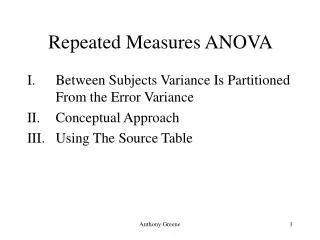
Effects • RMANOVA gives you 2 different kinds of effects • Within-Subjects effects • Between-Subjects effects • Interaction between the two
Within-Subjects Effects • This is the “true” repeated measures effect • Is there a mean difference between measurement occasions within my participants?
Between-Subjects Effects • These are the effects on IV’s that examine differences between different kinds of participants • All our effects from MANOVA are between-subjects effects • The IV itself is called a between-subjects factor
Mixed Effects • Mixed effects are another named for the interaction between a within-subjects factor and a between-subjects factor • Does the within-subjects effect differ by some between-subjects factor
EXAMPLE • Lets say Eric Kail does an intervention to improve the collegiality of his fellow IO students • He uses a pretest—intervention—posttest design • The DV is a subjective measure of collegiality • Eric had a hypothesis that this intervention might work differently depending on the participants GPA (high and low)
EXAMPLE • Within-Subjects effect = • Between-Subjects effect = • Mixed effect =
Within-Subjects RMANOVA • A within-subjects repeated measures ANOVA is used to determine if there are mean differences among the different time points • There is no between-subjects effect so we aren’t worried about anything BUT the WS effect • The within-subjects effect is an OMNIBUS test • We must do follow-up tests to determine which time points differ from one another
Example • 10 participants enrolled in a weight loss program • They got weighed when thy first enrolled and then each month for 2 months • Did the participants experience significant weight loss? And if so when?
You can name your within-subjects factor anything you want. “3” reflects the number of occasions
We also get to do post-hoc comparisons Just how was always do it!
c Multivariate Tests Partial Eta Noncent. Observed a Effect Value F Hypothesis df Error df Sig. Squared Parameter Power b occasion Pillai's Trace .590 5.751 2.000 8.000 .028 .590 11.502 .704 b Wilks' Lambda .410 5.751 2.000 8.000 .028 .590 11.502 .704 b Hotelling's Trace 1.438 5.751 2.000 8.000 .028 .590 11.502 .704 b Roy's Largest Root 1.438 5.751 2.000 8.000 .028 .590 11.502 .704 a. Computed using alpha = .05 b. Exact statistic c. Design: Intercept Within Subjects Design: occasion WHAT DOES THIS MEAN???
This is the previous 0.046 times 3 (for 3 comparisons)
Write Up • In order to determine if there was significant weight loss over the three occasions a repeated measures analysis of variance was conducted. Results indicated a significant within-subjects effect [F(1.29, 11.65) = 8.77, p < .05, η2=.49] indicating a significant mean difference in weight among the three occasions. As can be seen in Figure 1, the mean weight at month 2 and 3 was significantly lower relative to month 1 [F(1, 9) = 12.73, p < .05, η2=.58]. There was additional significant weight loss from month 2 to month 3 [F(1,9) = 5.38, p < .05, η2=.49.
Within and between-subject factors • When you have both WS and BS factors then you are going to be interested in the interaction! • IV = intgrp (4 levels) • DV = speed at pretest and posttest
GLM spdcb1 spdcb2 BY intgrp /WSFACTOR = prepost 2 Repeated /MEASURE = speed /METHOD = SSTYPE(3) /PLOT = PROFILE( prepost*intgrp ) /EMMEANS = TABLES(intgrp) COMPARE ADJ(BONFERRONI) /EMMEANS = TABLES(prepost) COMPARE ADJ(BONFERRONI) /EMMEANS = TABLES(intgrp*prepost) COMPARE(prepost) ADJ(BONFERRONI) /EMMEANS = TABLES(intgrp*prepost) COMPARE(intgrp) ADJ(BONFERRONI) /PRINT = DESCRIPTIVE ETASQ HOMOGENEITY /CRITERIA = ALPHA(.05) /WSDESIGN = prepost /DESIGN = intgrp .