Repeated Measures Designs
580 likes | 1.43k Vues
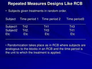
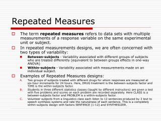
Repeated Measures Designs. In a Repeated Measures Design. We have experimental units that may be grouped according to one or several factors (the grouping factors) Then on each experimental unit we have not a single measurement but a group of measurements (the repeated measures)

Repeated Measures Designs
E N D
Presentation Transcript
In a Repeated Measures Design We have experimental units that • may be grouped according to one or several factors (the grouping factors) Then on each experimental unit we have • not a single measurement but a group of measurements (the repeated measures) • The repeated measures may be taken at combinations of levels of one or several factors (The repeated measures factors)
Example In the following study the experimenter was interested in how the level of a certain enzyme changed in cardiac patients after open heart surgery. • The enzyme was measured • immediately after surgery (Day 0), • one day (Day 1), • two days (Day 2) and • one week (Day 7) after surgery • for n = 15 cardiac surgical patients.
The data is given in the table below. Table: The enzyme levels -immediately after surgery (Day 0), one day (Day 1),two days (Day 2) and one week (Day 7) after surgery
The subjects are not grouped (single group). • There is one repeated measures factor -Time – with levels • Day 0, • Day 1, • Day 2, • Day 7 • This design is the same as a randomized block design with • Blocks = subjects
The Anova Table for Enzyme Experiment The Subject Source of variability is modelling the variability between subjects The ERROR Source of variability is modelling the variability within subjects
Example:(Repeated Measures Design - Grouping Factor) • In the following study, similar to example 3, the experimenter was interested in how the level of a certain enzyme changed in cardiac patients after open heart surgery. • In addition the experimenter was interested in how two drug treatments (A and B) would also effect the level of the enzyme.
The 24 patients were randomly divided into three groups of n= 8 patients. • The first group of patients were left untreated as a control group while • the second and third group were given drug treatments A and B respectively. • Again the enzyme was measured immediately after surgery (Day 0), one day (Day 1), two days (Day 2) and one week (Day 7) after surgery for each of the cardiac surgical patients in the study.
Table: The enzyme levels - immediately after surgery (Day 0), one day (Day 1),two days (Day 2) and one week (Day 7) after surgeryfor three treatment groups (control, Drug A, Drug B)
The subjects are grouped by treatment • control, • Drug A, • Drug B • There is one repeated measures factor -Time – with levels • Day 0, • Day 1, • Day 2, • Day 7
The Anova Table There are two sources of Error in a repeated measures design: The betweensubject error – Error1 and the withinsubject error – Error2
Tables of means Drug Day 0 Day 1 Day 2 Day 7 Overall Control 118.63 77.88 60.50 55.75 78.19 A 103.25 68.25 52.00 51.50 68.75 B 103.38 69.38 54.13 51.50 69.59 Overall 108.42 71.83 55.54 52.92 72.18
Example: Repeated Measures Design - Two Grouping Factors • In the following example , the researcher was interested in how the levels of Anxiety (high and low) and Tension (none and high) affected error rates in performing a specified task. • In addition the researcher was interested in how the error rates also changed over time. • Four groups of three subjects diagnosed in the four Anxiety-Tension categories were asked to perform the task at four different times patients in the study.
The number of errors committed at each instance is tabulated below.
Latin Square Designs Selected Latin Squares 3 x 34 x 4 A B C A B C D A B C D A B C D A B C D B C A B A D C B C D A B D A C B A D C C A B C D B A C D A B C A D B C D A B D C A B D A B C D C B A D C B A 5 x 56 x 6 A B C D E A B C D E F B A E C D B F D C A E C D A E B C D E F B A D E B A C D A F E C B E C D B A F E B A D C
Definition • A Latin square is a square array of objects (letters A, B, C, …) such that each object appears once and only once in each row and each column. Example - 4 x 4 Latin Square. A B C D B C D A C D A B D A B C
In a Latin square You have three factors: • Treatments (t) (letters A, B, C, …) • Rows (t) • Columns (t) The number of treatments = the number of rows = the number of colums = t. The row-column treatments are represented by cells in a t x t array. The treatments are assigned to row-column combinations using a Latin-square arrangement
Example A courier company is interested in deciding between five brands (D,P,F,C and R) of car for its next purchase of fleet cars. • The brands are all comparable in purchase price. • The company wants to carry out a study that will enable them to compare the brands with respect to operating costs. • For this purpose they select five drivers (Rows). • In addition the study will be carried out over a five week period (Columns = weeks).
Each week a driver is assigned to a car using randomization and a Latin Square Design. • The average cost per mile is recorded at the end of each week and is tabulated below:
The Model for a Latin Experiment i = 1,2,…, t j = 1,2,…, t k = 1,2,…, t yij(k) = the observation in ith row and the jth column receiving the kth treatment m = overall mean tk = the effect of the ith treatment No interaction between rows, columns and treatments ri = the effect of the ith row gj = the effect of the jth column eij(k) = random error
A Latin Square experiment is assumed to be a three-factor experiment. • The factors are rows, columns and treatments. • It is assumed that there is no interaction between rows, columns and treatments. • The degrees of freedom for the interactions is used to estimate error.
Example In this Experiment thewe are again interested in how weight gain (Y) in rats is affected by Source of protein (Beef, Cereal, and Pork) and by Level of Protein (High or Low). There are a total of t = 3 X 2 = 6 treatment combinations of the two factors. • Beef -High Protein • Cereal-High Protein • Pork-High Protein • Beef -Low Protein • Cereal-Low Protein and • Pork-Low Protein
In this example we will consider using a Latin Square design Six Initial Weight categories are identified for the test animals in addition to Six Appetite categories. • A test animal is then selected from each of the 6 X 6 = 36 combinations of Initial Weight and Appetite categories. • A Latin square is then used to assign the 6 diets to the 36 test animals in the study.
A represents the high protein-cereal diet • B represents the high protein-pork diet • C represents the low protein-beef Diet • D represents the low protein-cereal diet • E represents the low protein-pork diet and • F represents the high protein-beef diet. In the latin square the letter
The weight gain after a fixed period is measured for each of the test animals and is tabulated below:
Diet SS partioned into main effects for Source and Level of Protein
Graeco-Latin Square Designs Mutually orthogonal Squares
Definition A Greaco-Latin square consists of two latin squares (one using the letters A, B, C, … the other using greek letters a, b, c, …) such that when the two latin square are supper imposed on each other the letters of one square appear once and only once with the letters of the other square. The two Latin squares are called mutually orthogonal. Example: a 7 x 7 Greaco-Latin Square Aa Be Cb Df Ec Fg Gd Bb Cf Dc Eg Fd Ga Ae Cc Dg Ed Fa Ge Ab Bf Dd Ea Fe Gb Af Bc Cg Ee Fb Gf Ac Bg Cd Da Ff Gc Ag Bd Ca De Eb Gg Ad Ba Ce Db Ef Fc
Note: At most (t –1) t x t Latin squares L1, L2, …, Lt-1 such that any pair are mutually orthogonal. It is possible that there exists a set of six 7 x 7 mutually orthogonal Latin squares L1, L2, L3, L4, L5, L6 .
The Greaco-Latin Square Design - An Example • the percentage of Lysine in the diet and • percentage of Protein in the diet • have on Milk Production in cows. A researcher is interested in determining the effect of two factors Previous similar experiments suggest that interaction between the two factors is negligible.
For this reason it is decided to use a Greaco-Latin square design to experimentally determine the two effects of the two factors (Lysine and Protein). • Seven levels of each factor is selected • 0.0(A), 0.1(B), 0.2(C), 0.3(D), 0.4(E), 0.5(F), and 0.6(G)% for Lysine and • 2(a), 4(b), 6(c), 8(d), 10(e), 12(f) and 14(g)% for Protein ). • Seven animals (cows) are selected at random for the experiment which is to be carried out over seven three-month periods.
A Greaco-Latin Square is the used to assign the 7 X 7 combinations of levels of the two factors (Lysine and Protein) to a period and a cow. The data is tabulated on below:
The Model for a Greaco-Latin Experiment j = 1,2,…, t i = 1,2,…, t k = 1,2,…, t l = 1,2,…, t yij(kl) = the observation in ith row and the jth column receiving the kth Latin treatment and the lth Greek treatment
m = overall mean tk = the effect of the kth Latin treatment ll = the effect of the lth Greek treatment ri = the effect of the ith row gj = the effect of the jth column eij(k) = random error No interaction between rows, columns, Latin treatments and Greek treatments
A Greaco-Latin Square experiment is assumed to be a four-factor experiment. • The factors are rows, columns, Latin treatments and Greek treatments. • It is assumed that there is no interaction between rows, columns, Latin treatments and Greek treatments. • The degrees of freedom for the interactions is used to estimate error.
The Anova Table for a Greaco-Latin Square Experiment