Measuring clustering …
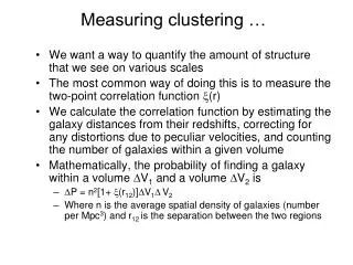
Measuring clustering …. We want a way to quantify the amount of structure that we see on various scales The most common way of doing this is to measure the two-point correlation function (r)

Measuring clustering …
E N D
Presentation Transcript
Measuring clustering … • We want a way to quantify the amount of structure that we see on various scales • The most common way of doing this is to measure the two-point correlation function (r) • We calculate the correlation function by estimating the galaxy distances from their redshifts, correcting for any distortions due to peculiar velocities, and counting the number of galaxies within a given volume • Mathematically, the probability of finding a galaxy within a volume V1 and a volume V2 is • P = n2[1+ (r12)]V1V2 • Where n is the average spatial density of galaxies (number per Mpc3) and r12 is the separation between the two regions
Measuring clustering … • P = n2[1+ (r12)]V1V2 • When (r) > 0, then galaxies are clustered (which is what we see) • On scales of < 50h-1 Mpc, we can parameterize the correlation function as a power-law: (r) ~(r/r0)- where >0 • Thus the probability of finding one galaxy within a distance r of another is significantly increased (over random) when r< r0. r0 is called the “correlation length”. • Note that the 2 point correlation function isn’t good for describing one-dimensional filaments or two-dimensional walls. We need 3 and 4 point correlation functions for those. Much harder! • From the SDSS: r0=6.1 +/- 0.2 h-1 Mpc, =1.75 over the scales 0.1 – 16 h-1 Mpc
Measuring clustering … • The Fourier transform of (r) is the power spectrum • P(k), P(k) = 4 (r) [sin(kr)/kr] r2dr • k is the wavenumber, small values of k correspond to large physical scales • P(k) has the dimensions of volume. It will be at maximum close to the radius r where (r ) drops to zero. • Roughly speaking the power spectrum is a power-law at large k (small physical scales) and turns over at small k (large physical scales) • We can combine information from different measurements (redshift surveys, CMB, Ly forest, weak lensing) to trace P(k) over a large range of physical scales • The power spectrum provides strong constraints on the amount and type of dark matter and dark energy in the universe
Measuring clustering … • We would also like to know how well the galaxies trace the mass distribution, or in other words how biased are the galaxies relative to the dark matter • We generally assume that the two densities are linearly related such that: • Let x= x/x be the density fluctuation of a given population • Linear biasing for galaxies implies galaxies=bdark matter • Biasing may be a function of scale and of galaxy luminosity • We can measure relative biasing by measuring the power spectrum of different populations
Peculiar velocities & Bulk Flows • Large scale structure causes peculiar velocities (different from the Hubble Flow) • We can measure these if we have accurate distances to the galaxies by: • Vr = H0d + Vpec – so if we measure distance and radial velocity (and assume the Hubble Constant) we can measure the peculiar velocity of a galaxy • We are moving towards the Virgo cluster at ~270 km/s, this is called the “Virgocentric infall” • We also measure a dipole anisotropy in the cosmic microwave background which implies that the local group is moving at ~620 km/s towards b=27, l=268. • This is due to a combination of our infall towards Virgo and the entire Local Supercluster moving towards the general direction of the Hydro-Centaurus Supercluster (the Great Attractor) • Flows of superclusters are known as “bulk flows” • Measurements of the velocity field of galaxies can help put constraints on the underlying mass field ==> measurement of dark matter over large scales
Dipole anisotropy in the Cosmic Microwave Background (from COBE 1992). We are moving wrt. to the CMB at ~620 km/s !!
Bulk flows, Aaronson et al 1986 Great Attractor
The GA lies in the “zone of avoidance”, it’s hard to study …
ACO 3627, Heart of the GA?
Dark Matter • Inventory of the universe --2008 WMAP (+BAO+SNe) results: • total=1.0052+/- 0.00064 (the universe is spatially flat!) • =0.721 +/- 0.0015 (but most of it is made of dark energy!) • matter=0.279 +/- 0.015 (and even the matter is confusing …) • baryon = 0.0462+/- 0.0015 but note that the baryon fraction observed in stars and gas is only * ~ 0.005 (so there must be some baryonic dark matter) • dark matter = 0.233 +/- 0.013 (and there is a LOT of non-baryonic matter!) • The evidence for dark matter has been with us significantly longer than that for dark energy, so the field is more mature. • There are lots of dark matter candidates, lots of fun for particle physicists! • But it’s always possible that we don’t understand gravity, so we need to modify gravity (MOND – Modified Newtonian Dynamics)
Evidence for Dark Matter • X-ray halos of Elliptical Galaxies • (Possibly) dynamics of globular clusters and planetary nebulae around elliptical galaxies (conflicting answers here!) • Flat rotation curves of spiral galaxies (best evidence!) • Kinematics of dwarf galaxies • Measurements of galaxy masses using “binary galaxies” • Measurements of the mass of galaxy clusters via: • X-ray gas • Motions • Gravitational lensing • Measurements on the largest scales from peculiar velocities
Measuring the mass from peculiar velocities • Assume that the measured peculiar velocities are generated locally • Then a galaxy only feels the gravitational pull of the nearest large mass concentration • The velocities are related to the local gravitational potential, which in turn is due to the mass distribution • Compare the observed velocity field to a density field (derived from a galaxy redshift survey) and derive the matter density distribution • Most results favor dark matter < 0.3. The universe cannot be flat (unless we have dark energy!)
Density contours from POTENT (Dekel 1994) and IRAS redshift survey (Strauss & Willick 1995)
HC Density contours from POTENT and IRAS redshift survey (Sigad et al. 1997)
Dark Matter (Baryonic) • Baryon inventory: from Big Bang nucleosynthesis calculations and the observations of light element abundances (deuterium, helium, and lithium) we can constrain baryon = 0.04 +/- 0.01 (more soon).This is the constraint from the very early universe, z~109. • These calculations are confirmed by the fluctuations in the Cosmic Microwave Background (again, more soon!)This measures baryon at z~1000. • And observations of the Ly forest – measures baryon at z~3. • Baryonic matter is made of stuff we understand – neutrons & protons (nucleons). • Everything we can observe directly is baryonic – stars, galaxies, hot x-ray gas, etc. • But today (z~0) we only observe = 0.0024 +/- 0.001 in cold stars and cold interstellar matter, and = 0.0026 in hot intracluster gas in clusters. • So we only directly observe ~12% of baryon at low redshift
Dark Matter (Baryonic) • What are the missing baryons? • Some candidates: • Some of it may be in low density warm/hot intergalactic medium (WHIM) that is difficult to measure (perhaps in the x-ray?) • Galaxies we don’t see (Low Surface Brightness Galaxies) • Cold dense clumps of hydrogen, of Jupiter-like masses ~10-3 M located in the halo. Microlensing surveys put strong constraints on the amount of mass that can be present in these clumps. Also unless they are reheated (by cosmic rays?) they would collapse. • Massive Compact Halo Objects (MACHOs) • White dwarfs • Brown dwarfs • Planets • Black holes (stellar remnants) • The list goes on, but we can place some observational constraints…
Dark Matter (Baryonic) • We can attempt to detect MACHOs via microlensing experiments • As a MACHO passes between us and a halo star, it will briefly amplify the light due to gravitational lensing • Need to continously monitor a large number of stars to search for such events, they are rare! • MACHO project started monitoring the LMC and fields in the Milky Way bulge from 1992 to 1999 using a 50 inch telescope at Mt. Stromlo observatory. • Other projects along these same lines include OGLE and AGAPE • Results indicate that machos may make up to 20% of the halo mass, the masses are similar to white dwarf masses
Dark Matter (Baryonic) • Some more “exotic” baryonic dark matter candidates: • Remnants of Pop III stars, very massive objects (VMOs) with M=103 – 106 M. These remnants might coalesce into one supermassive black hole (central engine of QSOs?) • But we would probably notice these if they were in the halo of the Milky Way as they would move in and out of the plane of the galaxy (~1 every 100 years or so) • Quantum black holes (primordial, created by quantum fluctuations in the very early universe) • These are tiny with M~1012 kg, r=10-13 cm • Probably not though …
Dark Matter (Non-Baryonic) • Most of the dark matter is non-baryonic • We need this dark matter to help turn density fluctuations in the early universe to the galaxies, clusters, filaments, walls, and voids we see today • Before recombination, baryonic dark matter interacted with radiation so the photons prevented the baryonic dark matter from collapsing to form structures.
COBE, extremely smooth blackbody T=2.725 K (error bars w/in thickness of the line!)
COBE, but there are small temperature fluctuations T/T ~ 10-5
Dark Matter (Non-Baryonic) • There are two types of non-baryonic dark matter: • Hot – matter is relativistic, so low-mass particles such as neutrinos. Their speed means they can escape from small density fluctuations, so if the DM is hot, small fluctuations dissolve and we don’t get enough structure on small scales. • So big structures form first (clusters), then later fragment to form galaxies. This is “top-down” structure formation. • Cold – matter moves more slowly. Exotic particles (not yet observed) such as axions, WIMPs, etc. Lots of fun for particle physicists! • Density fluctuations at all scales survive. Small fluctuations collapse first, then larger ones (pulling in the littler ones along the way). This is bottom-up structure formation and this is the best match to what we see today. • Note there is probably a little bit of hot (neutrinos have a non-zero mass) and a lot of cold dark matter.
Dark Matter (Non-Baryonic) • Cold Dark Matter (CDM) • Weakly interacting massive particles (WIMPs) – become non-relativistic at T > 104 K. Requires high masses up to 1016 GeV, 50-100 mass of proton. • WIMPs are found in supersymmetric (SUSY) theories of particle physics which predicts neutralinos, gravitinos, photinos, and higgsino • More recently the WIMPzilla has been introduced, 1010 x mass of WIMPS. These would have been created just after the Big Bang. These might explain high-energy cosmic rays. • Another possibility is axions, lighter masses 10-12 eV to 1 MeV • Axions predicted by quantum chromodynamics • No experimentally verified CDM candidates! Bummer!! LHC to the rescue?
Dark Matter (Non-Baryonic) • Hot Dark Matter (HDM) • Only form of non-baryonic matter known to exist • Must remain relativistic, which implies masses < 100 eV • Can find mass limits on the neutrino from ground-based neutrino experiments, as well as from the observed power spectrum of galaxies. These also place density limits as well. • neutrino = 0.001 – 0.05 (WMAP says < 0.003), so most of the dark matter must be cold!
Is gravity wrong? • Milgrom (1983) proposed a modification to Newtonian gravity, Modified Newtonian Dynamics (MOND) • F=m(a/a0)a where (x>>1) = 1 (normal gravity) and (x<<1) ~ x, so MOND would only kick in at low accelerations (what we generally see in galaxy dynamics) a0~10-8 cm/s2 • For a<< a0, a=sqrt(a0gN) there is more acceleration than expected from Newtonian gravity at slow acceleration scales • MOND can explain flat rotation curves and the Tully-Fisher relation • MOND can’t explain extra mass in the cores of big clusters (acceleration scales too big)