Download
1 / 60
600 likes | 628 Vues
Ascender II focuses on 3D geometric site model reconstruction using multiple images and sensors, applying context-sensitive control strategies and layered Bayesian networks for accurate results. It evaluates algorithms for building detection and geometric accuracy to improve site modeling outcomes.

E N D
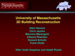
Allen HansonChris JaynesMauricio MarengoniEdward RisemanHoward SchultzFrank Stolle Ascona 2001 University of Massachusetts 3D Building Reconstruction With: Keith Hoepfner and Heddi Plumb
Talk Outline • Introduction: RADIUS and Ascender I • Overview of Ascender II • Geometric Reconstruction of Rooftops • Experiments • Conclusions Lab URL: http://vis-www.cs.umass.edu APGD URL: http://vis-www.cs.umass.edu/projects/ascender/ascender.html
Research Goal(s) 3D Geometric Site Model Reconstruction With multiple objects, Using multiple strategies, From multiple images EO, Digital Elevation Maps IFSAR, Multi/Hyperspectral
RADIUS: Ascender I System for Automatic Site Modelling Multiple Images Geometric Models • 2D polygon detection • line extraction • corner detection • perceptual grouping • epipolar matching • multi-image triangulation • geometric constraints • precise photogrammetry • extrusion to ground plane • projective texture mapping • CVIU 72(2) 1998
Ascender Works Detection Rates • Extensive evaluation • Good detection but high false alarms • Good geometric accuracy Ground Truth Ascender Results
Ascender Doesn’t Work • Delivered to NEL (NIMA) • Applied to classified imagery • Performance not as expected • High failure rate (buildings not detected) • High false positive rate • WHY? Imagery didn’t No Buildings Detected! conform to design constraints!
Some Observations • IU Algorithms work within correct context • constrained contexts • constrained object classes • Domain knowledge provides constraints • from domain, partial results, strategies • Many strategies, only correct ones used • selective application • correct parameters • fuse results from individual strategies into complete reconstruction
Key to Success A system which: applies the right strategy at the right time in the right place with the right constraints
Dealing with Context: Ascender II • Goals • 3D Geometric Site Model Reconstruction • Focus: More complex building structures • Context sensitive control strategies for applying algorithms • Multiple strategies • Multiple images • Multiple sensors • Knowledge Representation, Control and Inferencing • layered Bayesian networks EO, Digital Elevation Maps IFSAR, Multi/Hyperspectral
Where are the buildings? What is their structure? Observations Buildings = Location + Geometry Reconstruction = Localization + 3D Recovery 3D Recovery is a two-stage process
Ascender II Overview • IU Algorithms work within correct context. • Domain knowledge provides constraints. • Choose good strategy from many alternatives. CP: Control Policy Basic Principles
Ascender II Components • Visual Subsystem • Library of IU Algorithms • Geometric Database (data, models) • Display/user interface through RCDE • Knowledge Base • Control system • Belief networks in Hugin • Reasoning mechanisms over regions of discourse • Regions of Discourse • Subset of available data • Image regions, a model, partial interpretation
Schema/Belief Node Possible Values H1={j,..,k} Variable of interest H1 Evidence Policy H3 H2 First level of classification hierarchy H4 Second level (object subclass) Knowledge Representation • Combination of belief networks and • visual schemas, implemented in Hugin. • Encodes: Domain Knowledge • Acquired Site Knowledge • Control Mechanism • Allows both diagnostic and • causal inference. • Evidence policy defines how • IU strategies gather relevant • evidence according to context. • Hierarchical topology allows simpler • networks which reduces propagation • time and controls complexity.
Algorithms to Evidence Given an IU algorithm.... • Define the context in which it can run • currently straightforward • context only disallows an algorithm • too simple in the long run • Method for deriving certainty value • needed to update knowledge network
Algorithms • Algorithms operate on regions of discourse • Ascender I • Surface Fits • Line Extraction and Count • Junction Count • Average Junction Contrast • Region Height • Region Height to Width ratio • Edge Terminals • ……………...
Fusing DEM and Optical Data • Registered Optical and Elevation • Reconstruct Rooftops (and buildings) Optical Image (Fort Hood) Elevation Data (Fort Hood)
Technical Overview Registered Optical and DEM Model Indexing Parameterized Model Library Elevation Surface and Histogram Site Model Visualization Model Fit: Optimization
Surface Primitive Library 51 Models in 8 Parameterized Classes Gable
Experiments • Approach • Site model from Ascender I with no filtering and loose polygon acceptance criteria => high detection rate but lots of errors (false positives) • Classify Ascender I regions into {building, parking lot, open field, unknown} • Classify buildings into {multi-level building, single-level building} • Then into {flat, peak, round, flat-peak, other} • Site model from Ascender II after classification/reconstruction
20 False Positive Buildings Degraded Ascender I ModelFort Hood No Knowledge and Loose Polygon Acceptance Criteria A 22 True Positive Buildings 1 Incorrect Model (A) (multi-level reconstructed as single level)
First level of classification hierarchy Second level (object subclass) Bayes Nets for Experiments Level 1 Building Open Field Parking Lot Complex Unknown Region Evidence Policy: none Level 2 Low Medium High L Junctions Line Count Planar Fit Good Bad Multi-Level Building Width Height Single Evidence Policy: none Evidence Policy: Evidence Policy: multi-EO: triangulateHeight() DEM: medianHeight() DEM: robustFit(plane) Next Slide T Junctions Planar Fit Good Bad Yes No Evidence Policy: EO: junctions(T) <50 >50 Zero <5 >5 None Number T Junc. Contrast T Junc. Evidence Policy: Evidence Policy: EO: junction_count(T) EO: junction_contr(T)
Yes No Height A > Height B Yes No Center Line Ratio Level 3 of Network Level 3 Flat Peak Round Flat-peak Other Multiple calls, one for each section Rooftop Evidence Policy: none Level 3 Good Bad Yes No Yes No Middle > Corner Planar Fit Center Line Multi- level Yes No Evidence Policy: Prism Round Flat Yes No Evidence Policy: none Shadow Format DEM: robustFit(plane) Side Line Good Bad Good Bad Planar Fit B Planar Fit A Evidence Policy: Evidence Policy: DEM: robustFit(plane) DEM: robustFit(plane)
Height Visual Subsystem:Algorithms and Evidence Policies • Evidence policies associate algorithms with belief. • Function P maps request for evidence from knowledge base to algorithm. • F(x) maps algorithm result to belief value. • Example Algorithms: • Parallel Lines • T junctions • DEM-Median-Height • Region-Edge-Triangulate-Height • Planar Fit Error P{} P{} Height Stereo-Optical DEM DEM Median Height Multi-Optical Epipolar Align. Region-Edge Triangulate Hgt. USGS DTM DTM at region center F{x} x
Experiments • Detection rates per Object Class (Semantic Accuracy) • Three-Dimensional Accuracy • For each DataSet • For each Object Class (buildings) • How do network priors influence performance? • Uniform (no knowledge) versus Estimated Priors • Adjustment of Priors for each dataset versus uniform • Three Datasets • Fort Benning MOUT • Fort Hood Facility • Avenches Boat Yard
Priors and Operators Used Network Priors by Dataset Operators Applied by Dataset Skip F.Hood
43 Regions, 4 Misclassified, 1 Unknown 88% Accuracy Ascender II ClassificationContext Sensitive Strategies
Ascender II Reconstruction 3 False Positives 23 True Positive Buildings 0 Incorrect Models (single, multi level) 3 New Functional Areas
Reconstruction Accuracy:Fort Hood Detection Rates by Object Class Median Accuracy Measures , Building Classes Skip Avenches
ISPRS Avenches Dataset • Two Overlapping Optical Images (60% sideward) • Corresponding DEM • Calibration provided by ETH • 200x220 meter “Boatyard” • Ground Sample Dist: ~ 0.13 meters • Reference model provided by ETH
Regions and Classifications:Avenches P e a k B l d g . P e a k B l d g . F l a t B l d g . F l a t B l d g . F l a t B l d g . P a r k i n g L o t F l a t B l d g . F l a t B l d g . O p e n F i e l d P e a k B l d g . P e a k B l d g . P e a k B l d g .
Site Reconstruction:Avenches Skip Benning
Fort Benning MOUT Site Optical DEM • Two overlapping downlooking optical images • DEM computed from image pair using Terrest • Camera resection (SRI) • Reference Model (SRI) • GSD, optical view, 0.31 meters
MOUT Input Polygons Original Image Ascender I Polygons Final Polygons Polygons from SAR +
MOUT Site: Classification Flat roof building detected as peak. Low walled entrance (open field) Detected as single vehicle. Missed detection of two vehicles. Object Class True False False Positive Positive Negative Building (General) 19 1 0 Peak Roof 14 1 0 Flat Roof 5 0 0 Single Car 1 1 2 Recovery of 4 attached buildings. Overall classification accuracy: 91%
.939 .819 .742 .601 Plane Flat Peak Peak (15) Peak (35) Model Indexing: MOUT Region 8 Correlation Scores Corresponding Gaussian Sphere Constructed Surface Mesh
MOUT Site: Accuracy Detection Rates, Full Evaluation Detection Rates, FOA Regions Only
MOUT Reconstruction Skip Kodak
Hospital FineArts Examples on Three Image Chips Industrial N
Building FP Hypotheses Optical Lines 2D Polygons + Building FP Hypotheses Buildings (st. lines) Trees (no st. lines) v Elevation Blobs Building Localization Trees Buildings Ground Final Building Location Hypotheses Building FP Hypotheses + Classifier: Registration FP = Footprint
Geometric Recovery Building Localization: Polygons Canny Edges Grouped Lines Hypotheses Building Footprint On Range Data Polys Graph Group Focus (optional) Essentially Ascender I 2D Polygon Detection Algorithm with additional external inputs providing additional constraints. Classification
Building Localization: Blobs Thresholded using bald earth model Range Data First Threshold Filtered using Long Lines and Region Size Bald Earth Model Lines from Optical
Localization Results Hospital Industrial Fine Arts
Conclusions • Vision works when properly constrained and focused • Still a lot of work to do on: • Basic Algorithms • Knowledge Representations • Representing and Using Context and Constraints • Inferencing and Causal Reasoning • System Architectures