Expectation Maximization
Expectation Maximization. Dekang Lin Department of Computing Science University of Alberta. Objectives. Expectation Maximization (EM) is perhaps most often used and mostly half understood algorithm for unsupervised learning. It is very intuitive.

Expectation Maximization
E N D
Presentation Transcript
Expectation Maximization Dekang Lin Department of Computing Science University of Alberta
Objectives • Expectation Maximization (EM) is perhaps most often used and mostly half understood algorithm for unsupervised learning. • It is very intuitive. • Many people rely on their intuition to apply the algorithm in different problem domains. • I will present a proof of the EM Theorem that explains why the algorithm works. • Hopefully this will help applying EM when intuition is not obvious.
Model Building with Partial Observations • Our goal is to build a probabilistic model • A model is defined by a set of parameters θ • The model parameters can be estimated from a set of training examples: x1, x2, …, xn • xi’s are identically and independently distributed (iid) • Unfortunately, we only get to observe part of each training example: • xi=(ti, yi) and we can only observe yi. • How do we build the model?
Example: POS Tagging • Complete data: A sentence (a sequence of words) and a corresponding sequence of POS tags. • Observed data: the sentence • Unobserved data: the sequence of tags • Model: an HMM with transition/emission probability tables.
Training with Tagged Corpus • Pierre NNP Vinken NNP , , 61 CD years NNS old JJ , , will MD join VB the DT board NN as IN a DT nonexecutive JJ director NN Nov. NNP 29 CD . . • Mr. NNP Vinken NNP is VBZ chairman NN of IN Elsevier NNP N.V. NNP , , the DT Dutch NNP publishing VBG group NN . . • Rudolph NNP Agnew NNP , , 55 CD years NNS old JJ and CC former JJ chairman NN of IN Consolidated NNP Gold NNP Fields NNP PLC NNP , , was VBD named VBN a DT nonexecutive JJ director NN of IN this DT British JJ industrial JJ conglomerate NN . . • Pierre NNP Vinken NNP , , 61 CD years NNS old JJ , , will MD join VB the DT board NN as IN a DT nonexecutive JJ director NN Nov. NNP 29 CD . . • Mr. NNP Vinken NNP is VBZ chairman NN of IN Elsevier NNP N.V. NNP , , the DT Dutch NNP publishing VBG group NN . . • Rudolph NNP Agnew NNP , , 55 CD years NNS old JJ and CC former JJ chairman NN of IN Consolidated NNP Gold NNP Fields NNP PLC NNP , , was VBD named VBN a DT nonexecutive JJ director NN of IN this DT British JJ industrial JJ conglomerate NN . . c(JJ)=7 c(JJ, NN)=4, P(NN|JJ)=4/7
What is the best Model? • There are many possibly models • Many possible ways to set the model parameters. • We obviously want the “best” model. • Which model is the best? • The model that assigns the highest probability to the observation is the best. • Maximize Πi Pθ(yi), or equivalently Σi log Pθ(yi) • What about maximizing the probability of the hidden data? • This is know as the maximum likelihood estimation (MLE)
MLE Example • A coin with P(H)=p, P(T)=q. • We observed m H’s and n T’s. • What are p and q according to MLE? • Maximize Σi log Pθ(yi)= log pmqn • Under the constraint: p+q=1 • Lagrange Method: • Define g(p,q)=m log p + n log q+λ(p+q-1) • Solve the equations
Example • Suppose we have two coins. Coin 1 is fair. Coin 2 has probability p generating H. • They each have ½ probability to be chosen and tossed. • The complete data is (1, H), (1, T), (2, T), (1, H), (2, T) • We only know the result of the toss, but don’t know when coin was chosen. • The observed data is H, T, T, H, T. • Problem: • Suppose the observations include m H’s and n T’s. • How to estimate p to maximize Σi log Pθ(yi)?
Need for Iterative Algorithm • Unfortunately, we often cannot find the best θ by solving equations. • Example: • Three coins, 0, 1, and 2, with probabilities p0, p1, and p2 generating H. • Experiment: Toss coin 0 • If H, toss coin 1 three times • If T, toss coin 2 three times • Observations: • <HHH>, <TTT>, <HHH>, <TTT>, <HHH> • What is MLE for p0, p1, and p2?
Overview of EM • Create an initial model, θ0. • Arbitrarily, randomly, or with a small set of training examples. • Use the model θ’ to obtain another model θ such that Σi log Pθ(yi) > Σi log Pθ’(yi) • Repeat the above step until reaching a local maximum. • Guaranteed to find a better model after each iteration.
Maximizing Likelihood • How do we find a better model θ given a model θ’? • Can we use Lagrange method to maximize ΣilogPθ(yi)? • If this can be done, there is no need to iterate!
EM Theorem • The following EM Theorem holds • This theorem is similar to (but is not identical to, nor does it follow) the EM Theorem in [Jelinek 1997, p.148] (the proof is almost identical). • EM Theorem: Σt is summation over all possible values of unobserved data
What does EM Theorem Mean? • If we can find a θ that maximizes the same θ will also satisfy the condition which is needed in the EM algorithm. • We can maximize the former by taking its partial derivatives w.r.t. parameters in θ.
EM Theorem: why? • Why optimizing is easier than optimizing • Pθ(t, yi) involves the complete data and is usually a product of a set of parameters. Pθ(yi) usually involves summation over all hidden variables.
EM Theorem: Proof =1 ≤0 (Jensen’s Inequality)
The proof used the inequality • More generally, if p and q are probability distributions • Even more generally, if f is a convex function, E[f(x)] ≥ f(E[x]) • Jensen’s Inequality
What is ? • The expected value of log Pθ(t,yi) according to the model θ’. • The EM Theorem states that we can get a better model by maximizing the sum (over all instances) of the expectation.
A Generic Set Up for EM • Assume Pθ(t, y) is a product of a set of parameters. • Assume θ consists of M groups of parameters. • The parameters in each group sum up to 1. • Let ujk be a parameter. Σmujm=1 • Let Tjk be a subset of hidden data such that if t is in Tjk, the computation of Pθ(t, yi) involves ujk. • Let n(t,yi) be the number of times ujk is used in Pθ(t,yi), i.e., Pθ(t,yi)=ujkn(t,yi)v(t,y), where v(t,y) is the product of all other parameters.
pseudo count of instances involving ujk
Summary • EM Theorem • Intuition • Proof • Generic Set-up

