A Hidden Markov Model Framework for Multi-target Tracking
A Hidden Markov Model Framework for Multi-target Tracking. DeLiang Wang Perception & Neurodynamics Lab Ohio State University. Outline. Problem statement Multipitch tracking in noisy speech Multipitch tracking in reverberant environments Binaural tracking of moving sound sources

A Hidden Markov Model Framework for Multi-target Tracking
E N D
Presentation Transcript
A Hidden Markov Model Frameworkfor Multi-target Tracking DeLiang Wang Perception & Neurodynamics Lab Ohio State University
Outline Problem statement Multipitch tracking in noisy speech Multipitch tracking in reverberant environments Binaural tracking of moving sound sources Discussion & conclusion 2
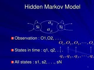
Multi-target tracking problem Multi-target tracking is a problem of detecting multiple targets of interest over time, with each target being dynamic (time-varying) in nature The input to a multi-target tracking system is a sequence of observations, often noisy Multi-target tracking occurs in many domains, including radar/sonar applications, surveillance, and acoustic analysis 3
Approaches to the problem Statistical signal processing has been heavily employed for the multi-target tracking problem In a very broad sense, statistical methods can be viewed Bayesian tracking or filtering Prior distribution describing the state of dynamic targets Likelihood (observation) function describing state-dependent sensor measurements, or observations Posterior distribution describing the state given the observations. This is the output of the tracker, computed by combining the prior and the likelihood 4
Kalman filter Perhaps the most widely used approach for tracking is a Kalman filter For linear state and observation models, and Gaussian perturbations, the Kalman filter gives a recursive estimate of the state sequence that is optimal in the least squares sense The Kalman filter can be viewed as a Bayesian tracker 5
General Bayesian tracking When the assumptions of the Kalman filter are not satisfied, a more general framework is needed For multiple targets, multiple hypothesis tracking or unified tracking can be formulated in the Bayesian framework (Stone et al.’99) Such general formulations, however, require an exponential number of evaluations, hence computationally infeasible Approximations and hypothesis pruning techniques are necessary in order to make use of these methods 6
Domain of acoustic signal processing Domain knowledge can provide powerful constraints to the general problem of multi-target tracking We consider the domain of acoustic/auditory signal processing, in particular Multipitch tracking in noisy environments Multiple moving-source tracking In this domain, hidden Markov model (HMM) is a dominant framework, thanks to its remarkable success in automatic speech recognition 7
HMM for multi-target tracking We have explored and developed a novel HMM framework for multi-target tracking for the problems of pitch and moving sound tracking (Wu et al., IEEE T-SAP’03; Roman & Wang, IEEE T-ASLP’08; Jin & Wang, OSU Tech. Rep.’09) Let’s first consider the problem of multi-pitch tracking 8
What is pitch? • “The attribute of auditory sensation in terms of which sounds may be ordered on a musical scale.” (American Standards Association) • Periodic sound: pure tone, voiced speech (vowel, voiced consonant), music • Aperiodic sound with pitch sensation, e.g. comb-filtered noise
Pitch of a periodic signal Fundamental Frequency (period) Pitch Frequency (period) d
Applications of pitch tracking • Computational auditory scene analysis (CASA) • Source separation in general • Automatic music transcription • Speech coding, analysis, speaker recognition and language identification
Existing pitch tracking algorithms • Numerous pitch tracking, or pitch determination algorithms (PDAs), have been proposed (Hess’83; de Cheveigne’06) • Time-domain • Frequency-domain • Time-frequency domain • Most PDAs are designed to detect single pitch in noisy speech • Some PDAs are able to track two simultaneous pitch contours. However, their performance is limited in the presence of broadband interference
Multipitch tracking in noisy environments Voiced signal Output pitch tracks Background noise Multipitch tracking Voiced signal
Diagram of Wu et al.’03 Normalized Correlogram Channel Selection Speech/ Interference Cochlear Filtering HMM-based Multipitch Tracking Channel Integration Continuous Pitch Tracks
Periodicity extraction using correlogram Normalized Correlogram High frequency Frequency channels Low frequency Delay Response to clean speech
Channel selection • Some frequency channels are masked by interference and provide corrupting information on periodicity. These corrupted channels are excluded from pitch determination (Rouat et al.’97) • Different strategies are used for selecting valid channels in low- and high-frequency ranges
HMM formulation Normalized Correlogram Channel Selection Speech/ Interference Cochlear Filtering HMM-based Multipitch Tracking Channel Integration Continuous Pitch Tracks
Pitch state space The state space of pitch is neither a discrete nor continuous space in a traditional sense, but a mix of the two (Tokuda et al.’99) Considering up to two simultaneous pitch contours, we model the pitch state space as a union of three subspaces: Zero-pitch subspace is an empty set: One-pitch subspace: Two-pitch subspace: 18
How to interpret correlogram probabilistically? The correlogram dominates the modeling of pitch perception (Licklider’51), and is commonly used in pitch detection We examine the relative time lag between the true pitch period and the lag of the closest peak True pitch delay (d) Peak delay (l) 19
Relative time lag statistics histogram from natural speech for one channel
Modeling relative time lags From the histogram data, we find that a mixture of a Laplacian and a uniform distribution is appropriate q is a partition coefficient The Laplacian models a pitch event and the uniform models “background noise” The parameters are estimated using ML from a small corpus of clean speech utterances 21
Modeling relative time-lag statistics Estimated probability distribution of (Laplacian plus uniform distribution)
One-pitch hypothesis First consider one-pitch state subspace, i.e. For a given channel, c, let denote the set of correlogram peaks If c is not selected, the probability of background noise is assigned 23
One-channel observation probability Normalized Correlogram 24
Integration of channel observation probabilities • How to integrate the observation probabilities of individual channels to form a frame-level probability? • Modeling joint probability is computationally prohibitive. Instead, • First we assume channel independence and take the product of observation probabilities of all channels • Then flatten (smooth) the product probability to account for correlated responses of different channels, or to correct the probability overshoot phenomenon (Hand & Hu’01)
Two-pitch hypothesis Next consider two-pitch state subspace, i.e. If channel energy is dominated by one source, d1 denotes relative time-lag distribution from two-pitch frames 26
Two-pitch hypothesis (cont.) By a similar channel integration scheme, we finally obtain This gives the larger of the two assuming either d1 or d2 dominates 27
Two-pitch integrated observation probability Pitch Delay 2 Pitch Delay 1 28
Zero-pitch hypothesis Finally consider zero-pitch state subspace, i.e. We simply give it a constant likelihood 29
HMM tracking Observed signal Observation probability Pitch state space Pitch dynamics One time frame 30
Prior (prediction) and posterior probabilities Prior probability for time frame m Assuming pitch period d for time frame m-1 d Observation probability for time frame m Posterior probability for time frame m d d 31
Transition probabilities • Transition probabilities consist of two parts: • Jump probabilities between pitch subspaces • Pitch dynamics within the same subspace • Jump probabilities are again estimated from the same small corpus of speech utterances • They need not be accurate as long as diagonal values are high
Pitch dynamics in consecutive time frames • Pitch continuity is best modeled by a Laplacian • Derived distribution consistent with the pitch declination phenomenon in natural speech (Nooteboom’97) 33
Search and efficient implementation • Viterbi algorithm is used to find the optimal sequence of pitch states • To further improve computational efficiency, we employ • Pruning: search only in a neighborhood of a previous pitch point • Beam search: search for a limited number of most probable state sequences • Search for pitch periods near local peaks
Evaluation results • The Wu et al. algorithm was originally evaluated on mixtures of 10 speech utterances and 10 interferences (Cooke’93), which have a variety including broadband noise, speech, music, and environmental sounds • The system generates good results, substantially better than alternative systems • The performance is confirmed by subsequent evaluations by others using different corpora
Example 1: Speech and white noise Tolonen & Karjalainen’00 Wu et al.’03 Pitch Period (ms) Time (s) Time (s)
Example 2: Two utterances Tolonen & Karjalainen’00 Wu et al.’03 Pitch Period (ms) Time (s) Time (s)
Outline Problem statement Multipitch tracking in noisy speech Multipitch tracking in reverberant environments Binaural tracking of moving sound sources Discussion & conclusion 38
Multipitch tracking for reverberant speech • Room reverberation degrades harmonic structure, making pitch tracking harder Mixture of two anechoic utterances Corresponding reverberant mixture
What is pitch of a reverberant speech signal? • Laryngograph provides ground truth pitch for anechoic speech. However, it does not account for fundamental alteration to the signal by room reverberation • True to the definition of signal periodicity and considering the use of pitch for speech segregation, we suggest to track the fundamental frequency of the quasi-periodic reverberant signal itself, rather than its corresponding anechoic signal (Jin & Wang’09) • We use a semi-automatic pitch labeling technique (McGonegal et al.’75) to generate reference pitch by examining waveform, autocorrelation, and cepstrum
HMM for multipitch tracking in reverberation We have recently applied the HMM framework of Wu et al.’03 to reverberant environments (Jin & Wang’09) The following changes are made to account for reverberation effects: A new channel selection method based on cross-channel correlation Observation probability is formulated based on a pitch saliency measure, rather than relative time-lag distribution which is very sensitive to reverberation These changes result in a simpler HMM model! Evaluation and comparison with Wu et al.’03 and Klapuri’08 show that this system is robust to reverberation, and gives better performance 41
Two-utterance example Upper: Wu et al.’03; lower: Jin & Wang’09 Reverberation time is 0.0 s (left), 0.3 s (middle), 0.6 s (right)
Outline Problem statement Multipitch tracking in noisy speech Multipitch tracking in reverberant environments Binaural tracking of moving sound sources Discussion & conclusion 43
HMM for binaural tracking of moving sources Binaural cues (observations) are ITD (interaural time difference) and IID (interaural intensity difference) The HMM framework is similar to that of Wu et al.’03 Roman & Wang (2008) 44
Likelihood in one-source subspace Joint distribution of ITD-IID deviations for one channel: Actual ITD Reference ITD 45
Three-source illustration and comparison Kalman filter output 46
Summary of moving source tracking The HMM framework automatically provides the number of active sources at a given time Compared to a Kalman filer approach, the HMM approach produces more accurate tracking Localization of multiple stationary sources is a special case The proposed HMM model represents the first CASA study addressing moving sound sources 47
General discussion The HMM framework for multi-target tracking is a form of Bayesian inference (tracking) that is broader than Kalman filtering Permits nonlinearity and non-Gaussianity Yields the number of active targets at all times Corpus-based training for parameter estimation Efficient search Our work has investigated up to two (pitch) or three (moving sources) target tracks in the presence of noise Extension to more than three is straightforward theoretically, but complexity becomes an issue increasingly However, for the domain of auditory processing, little need to track more than 2-3 targets due to limited perceptual capacity 48
Conclusion We have proposed an HMM framework for multi-target tracking State space consists of a discrete set of subspaces, each being continuous Observations (likelihoods) are derived in time-frequency domains: Correlogram for pitch and cross-correlogram for azimuth We have applied this framework to tracking multiple pitch contours and multiple moving sources The resulting algorithms perform reliably and outperform related systems The proposed framework appears to have general utility for acoustic (auditory) signal processing 49
Collaborators Mingyang Wu, Guy Brown Nicoleta Roman Zhaozhang Jin 50