Download
1 / 21
210 likes | 542 Vues
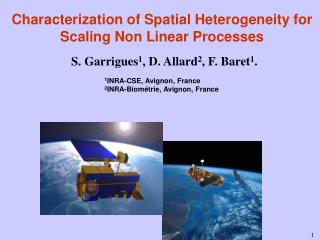
Characterization of Spatial Heterogeneity for Scaling Non Linear Processes . S. Garrigues 1 , D. Allard 2 , F. Baret 1 . 1 INRA-CSE, Avignon, France 2 INRA-Biométrie, Avignon, France. 1. Background. Sensor function. Reflectance Image ( {R i , i=1..n} ).

E N D
Characterization of Spatial Heterogeneity for Scaling Non Linear Processes S. Garrigues1, D. Allard2, F. Baret1. 1INRA-CSE, Avignon, France 2INRA-Biométrie, Avignon, France
1. Background Sensor function Reflectance Image ({Ri, i=1..n}) Different spatial and temporal scales Transfer Function BV = f(Ri) Biophysical variable (LAI, FAPAR) Vegetation monitoring at global scale (primary production, carbon cycle...) Vegetation ground scene (different biome types) Technological constraints: Coarse spatial resolution sensor Non linear process Need of high time frequency data
2. Problematic Puechabon: Woody savana Alpilles: Cropland Alpilles: Cropland Puechabon: Woody savana Nezer: Pine forest Counami: Tropical forest Counami: Tropical forest Nezer: Pine forest Image spatial structure depends on vegetation type 20m SPOT NDVI image
2. Problematic Puechabon: Woody Savana Alpilles: Cropland Nezer: Pine Forest Counami: Woody Savana Image spatial structure depends on vegetation type
20m (SPOT) 60m ( SPECTRA) Spatial Resolution 300m ( MERIS) 500m ( MODIS) 1000m ( VGT) 2. Problematic Image spatial structure depends on sensor spatial resolution « Homogeneous » (Guyana Forest) « Heterogeneous site » (Alpilles Cropland ) • The sensor integrates the signal over the pixel; intra-pixel variance lost • Spatial heterogeneity depends on the spatial resolution
Non linear transfer function between NDVI and LAI: LAI=f(NDVI) Heterogeneous pixel A B LAIB Apparent LAI LAIactual biais LAIapparent Bias: e=LAIapparent-LAIactual LAIA Actual LAI : NDVIA NDVIB NDVI 2. Problematic Spatial heterogeneity and non linear process
2. Problematic • Spatial structure (i.e. spatial heterogeneity) depends on: • surface property variation • sensor regularization • spatial characteristics: spatial resolution, support geometry (PSF), • viewing angle… • spectral characteristic, atmospheric effects • image extent • Working scale: the field scale Utilisation of high spatial resolution (SPOT 20m) to characterize ground spatial structure at field spatial frequency. • Spatial heterogeneity definition: • quantitative information characterizing the ground spatial structure • spatial variance distribution of the variable considered, within the coarse resolution pixel • Our aim:using spatial heterogeneity as an a priori information to correct biophysical estimation biais, i.e. to scale up the transfer function at coarser spatial resolution
3. Spatial heterogeneity characterization Stochastic framework for image exploitation • The image is a realization of a random process (random function model) with the following characteristics: • Ergodicity:one realization of the random process allows to infer the statistical properties of the random function. • Stationarity of the two first moments: • - the mean image value is constant over the image • - the correlation between two pixel values depends only on the distance between them. • Data support: SPOT pixel considered as punctual • No accounting for SPOT regularization (PSF) • No accounting for SPOT pixel radiometric uncertainties (measurement errors) • Variable studied : NDVI
Sample variogram: Sill (²) True Variance Sill(²) • Theoretical variogram Range (r) Up to this distance data are spatially correlated • Variogram regionalization model of the image: nested structure Range2 (r2) Range1 (r1) Standard variogram structure characterizes a spatial variation of the image 3. Spatial heterogeneity characterization The variogram: a structure function • Definition: • spatial variance distribution of the regionalized variable z(x)
Alpilles,r1=264m, r2=1148m, sill=0.042 Puechabon r1=260m, r2=1806m, sill=0.012 Nezer,r1=222m, r2=1533m, sill=0.0037 Counami,r1=57m, r2=676m, sill=0.00086 The variogram describes the ground spatial structure of different vegetation types. 3. Spatial heterogeneity characterization Spatial structure characterization by the variogram
Variance 3. Spatial heterogeneity characterization Spatial heterogeneity typology Integral range Integral range is a yardstick that summarizes variogram on the image
Image structure Ground structure Point Spread Function Regularized variogram Regularized variogram Ground variogram 4. Spatial heterogeneity regularization with decreasing spatial resolution Spatial structure regularization is a function of sensor spatial characteristics Sensor regularization Puechabon site
Sample dispersion variance Cropland Woody Savana Pixel x,Z(x) Pine forest Pixel vi, Z(vi) Tropical Forest • Theoretical dispersion variance: • Our model of data regularization • Quantify spatial heterogeneity (spatial variance) with spatial resolution 4. Spatial heterogeneity regularization with decreasing spatial resolution Spatial heterogeneity quantification
Biased LAI Sample dispersion variance Non linearity degree Heterogeneity degree 5 Bias correction model Univariate Model
5. Bias correction model Cropland site (Alpilles) example Resolution=500m Model problem: • Non stationnarity pixel: sample dispersion variance (pixel spatial heterogeneity) is lower than theoretical variance dispersion predicted by variogram model
5. Bias correction model Cropland site (Alpilles) example Resolution=500m Model problem: • Non stationnarity pixel: the sample dispersion variance of the pixel is lower than the theoretical variance dispersion predicted by the variogram model
5. Bias correction model Cropland site (Alpilles) example Resolution=1000m
6. Multivariate spatial heterogeneity characterization Multivariate description of spatial heterogeneity Coregionalization variogram model Alpilles (Cropland) • multi-spectral spatial heterogeneity • description: • more information on physical signal • using variance-covariance dispersion matrix to correct bias • Problems: disturbing factors (atmosphere) influence the spatial structure
5. Conclusions and prospects • Using variograms to describe spatial heterogeneity : • it describes the spatial structure of different landscapes • it allows to model data regularization • Bias correction model : • based on variogram models and accounts for the non linearity of the transfer function • allows accounting for actual PSF (sensor spatial characteristics, registration for data fusion) • Problems: • How to adjust variogram models for bias correction? • Temporal stationnarity of the variogram models? • Transfer function diversity: development of a multivariate model • Accounting for image spatial information for quantitative remote sensing is an important concern • Use of SPECTRA data to adjust variogram models and investig • ate their temporal stationnarity • Optimizing the PSF design of future missions
B LAI=f(NDVI) R^ C LAIb RV LAIR LAIh D A NDVIP NDVIA NDVIB Raffy Method – Univariate case
Heterogeneous pixel A B Apparent LAI LAIactual biais LAIapparent Bias: e=LAIapparent-LAIactual LAIA Actual LAI : NDVIA NDVI 2. Problematic Spatial heterogeneity and non linear process Non linear transfer function between NDVI and LAI: LAI=f(NDVI) LAIB NDVIB