Download
1 / 20
200 likes | 318 Vues
Spatial Heterogeneity and the Geographic Distribution of Airport Noise. ASSA Meeting – January 2010 Atlanta, GA. Jeffrey P. Cohen Associate Professor of Economics University of Hartford. Cletus C. Coughlin Vice President and Deputy Director of Research Federal Reserve Bank of St. Louis.

E N D
Spatial Heterogeneity and the Geographic Distribution of Airport Noise ASSA Meeting – January 2010 Atlanta, GA Jeffrey P. Cohen Associate Professor of Economics University of Hartford Cletus C. Coughlin Vice President and Deputy Director of Research Federal Reserve Bank of St. Louis • The authors thank Lesli Ott for excellent research assistance and the Atlanta Department of Aviation for noise contour data. We thank meeting participants at the Federal Reserve System Committee on Regional Economic Analysis, especially Anil Kumar, for their comments. Nancy Lozano-Gracia also provided helpful comments on an earlier version of the paper. The views expressed are those of the authors and do not necessarily reflect official positions of the Federal Reserve Bank of St. Louis, the Federal Reserve System, or the Board of Governors.
Motivation & Major Questions Motivation Possibility that airport noise depends on • neighborhood demographic characteristics • proximity to airport (noise and distance are not necessarily correlated) • prices of houses Major Questions • Which of the preceding variables are significant determinants of noise? Does estimation incorporating spatial heterogeneity generate results that differ from estimation ignoring spatial heterogeneity? • How do the results differ across locations? Why?
Approach Our approach • Locally Weighted Regressions (LWR) (non-parametric spatial specification) • This is opposed to spatial autocorrelation and/or spatially lagged variables (parametric approach) Advantage of LRW • Allows for non-uniformity in relationships between variables
Background: Airport Noise Federal Register (2000) Annoyance: the adverse psychological response to noise • 12 percent of people subjected to a DNL of 65 decibels report that they are “highly annoyed” • 3 percent are highly annoyed when subjected to a DNL of 55 decibels • 40 percent are highly annoyed at a DNL of 75 decibels Nelson (2004) Since 1979 federal agencies have regarded land subject to 65 to 74 decibels as “normally” incompatible with residential use and land subject to less than 65 decibels as “normally” compatible with residential land use
Airport Noise, Proximity & Housing Prices • Standard finding is that airport noise reduces housing prices: • McMillen (2004): 9 percent reduction for houses near Chicago O’Hare for 65 db or more • Over time, noise levels around O’Hare have decreased • Espey and Lopez (2000): 2 percent reduction for houses near Reno Cannon for 65 db or more • Lipscomb (2003): no effect for houses in College Park, GA, which is near Atlanta Hartsfield-Jackson • Proximity: must control for proximity to accurately measure effect of noise • Proximity tends to have a positive effect: • Tomkins, Topham, Twomey, and Ward (1998): Manchester • McMillen (2004): O’Hare • Lipscomb (2003): Hartsfield-Jackson
Other Studies of Airport Noise Cohen and Coughlin (2008): Atlanta, GA airport • noise assumed to be exogenous – common assumption • houses exposed to 70 db noise faced sale prices that were 20 percent lower than houses in the buffer zone Sobotta, et. al. (2007): Phoenix, AZ airport • modeled noise as dependent variable • found higher Hispanic neighborhoods were exposed to significantly more noise
Model • Estimation by Ordered Probit
Ordered Probit For ordered probit we re-define noise:
Alternative Estimation Approach Locally Weighted Regressions (LWR) • addresses spatial nature of the data Background • Spatial Econometrics (parametric approach) • LWR (non-parametric approach)
Locally Weighted Regressions (LWR) More tractable for ordered probit Advantages • non-parametric approach to address spatial variation • allows for non-linearity in relationships between independent variables and dependent variables • for ordered probit, can be estimated by a “pseudo maximum likelihood” approach
Locally Weighted Regressions (LWR) With 3 regimes in ordered probit, pseudo log-likelihood function is: where is standard normal c.d.f. is parameter vector for observation I Doj = 1 if obs. j = 0, = 0 otherwise D1j = 1 if obs. j = 1, = 0 otherwise D2j = 1 if obs. j = 2, = 0 otherwise • impact of spatial weights enters in a non-parametric way
Weights Somewhat different – we use Gaussian weight function: where is standard normal density function = distance between house i and house j = standard deviation of distances between house i and all other houses j = bandwidth • We use cross-validation to choose preferred b: • vary b to be 0.4, 0.6, 0.8, 1.0 • b = 0.4 maximizes the pseudo log-likelihood function
Data Atlanta airport Noise Contours: Atlanta Department of Aviation Housing Prices & Characteristics: 2003 Demographics: % Hispanic, % black, median household income from U.S. Census Bureau, 2000.
Comparison of OP and OPLWR Results 1 Parameter estimates with t-statistics in parenthesis. 2 The average of the 508 parameter estimates for the variable is listed on the first of the three lines, the standard deviation in parenthesis is on the middle line, and the range of parameter estimates in brackets is provided on the third line. The log-likelihood value is the sum of the log likelihoods for the 508 regressions. Bandwidth = 0.4.
OPLWR • Heterogeneity in the parameters for different houses • Sign switches: • log of distance • % Hispanic in block group • Examine the geographic aspects of these variables more clearly
Distance Coefficients and Location of Houses b = .4 b = .8
Hispanic Coefficients and Location of Houses Positive Coefficients Negative Coefficients
Conclusions • spatial effects matter • ignoring them can lead to biased results of assessing determinants of noise • find evidence of heterogeneity in effects of Hispanic population, and distance from airport, on probability of being in the “buffer zone”