Spatial and Geographic Databases
Spatial and Geographic Databases. Database extensions. Database management research is continuously expanding its scope of applicability Problems encountered: What is the next killer-application ? Technical problems: The old datatypes {int…str} are insufficient


Spatial and Geographic Databases
E N D
Presentation Transcript
Database extensions • Database management research is continuously expanding its scope of applicability • Problems encountered: • What is the next killer-application ? • Technical problems: • The old datatypes {int…str} are insufficient • The algorithms are often more complex than relation algebra • Application programmers treat data management equal to datastructures and algorithmic control
Case study: Sequoia benchmark • Sequoia Benchmark (1995-2000) • Presents a benchmark for earth science (ES) databases • A functional benchmark can be used to elucidate the requirements and describes the challenges in concrete terms: • Benchmark data • Benchmark query • Benchmark constraints and reporting
Case study: Sequoia benchmark • Satellite imagery (longitude, latitude, wavelength band, time); • Sample Earth’s surface on a 30m x 30m grid, in 7 wavelength bands, every 15 days. • Massive size: SEQUOIA 2000 ES – 100Tbytes of data NASA Earth Observation System – 10 petabytes • Complex data types: ES DBs include multi-dimensional arrays, geometries for spatial objects, and other complex data types. • Sophisticated searching: Searching arrays and spatial data for desired information.
Case study: Sequoia benchmark • Benchmark Data • Regional, National, World Benchmarks Raster Data: • RASTER (time, location, band, data) Point Data: • POINT (name, location) Polygon Data: • POLYGON (landuse, location) Directed Graph Data: • GRAPH (identifier, segment)
Case study: Sequoia benchmark Data Load ES expend much effort loading new data, this activity is usually disregarded in other benchmarks. Query 1: Create and load the data base and build any necessary secondary indexes. Query will record the elapsed time to load the data into the system being tested, performing whatever data conversions are desired, and building any secondary indexes.
Case study: Sequoia benchmark Raster Queries Query 2: Select RASTER data for a given wavelength band and rectangular region ordered by ascending time. Time travel query, watch what happens to as time increased. Query 3: Select RASTER data for a given time and geographic rectangle and then calculate an arithmetic function of the five wavelength band values for each cell in the study rectangle. Computes a weighted average of the individual cell values in data. The result for the function can not be pre-computed.
Case study: Sequoia benchmark • Query 4: Select RASTER data for a given time, wavelength band, and geographic rectangle. Lower the resolution of the image by a factor of 64 to a cell size of 4km x 4km and store it as a new DBMS object. • Changes the spatial resolution of a raster image, this operation creates an abstract of raster data. • It is useful to see a large area in low resolution and then zoom into areas of particular interest. • Requires dynamic creation of new DB tables/classes
Case study: Sequoia benchmark Point and Polygon Queries Query 5: Find the POINT record that has a specific name. System must have non-spatial indexing (B-tree, hashing) and be able to assemble spatial and non-spatial attributes for output. Query 6: Find all polygons that intersect a specific rectangle and store them in the DBMS. Requires spatial index (R-tree) and dynamic creation of new DB tables/classes
Case study: Sequoia benchmark • Point and Polygon Query • Query 7: Find all polygons that are more than a specific size and within a specific circle • Combination query that has both spatial/non-spatial restrictions. (R-tree) • Requirements • Query optimizer that can evaluate expected selectivity of spatial/non-spatial clause and choose the more restrictive one to process • The clause that spatially subsets the data should be used
Case study: Sequoia benchmark Spatial Joins Queries that join data of one spatial type to those of a different spatial type. Query 8: Show the landuse/landcover in a 50 km quadrangle surrounding a given point Find polygons that intersect a rectangle of interest. (R-tree) Perform complex spatial joins of POINT and POLYGON data sets
Case study: Sequoia benchmark Spatial Joins Query 9: Find the raster data for a given landuse type in a study rectangle for a given wavelength band and time Perform a join between raster data and polygon data Query 10: Find the names of all points within polygons of a specific vegetation type and create this as a new DBMS object. Join between point and polygon data. Dynamic creation of new DB tables/classes
Case study: Sequoia benchmark • Recursion • Need to trace drainage basins or irrigation networks à restricted recursive queries on network data • Query 11: Find all segments of any waterway that are within 20 km downstream of a specific geographic point • Computation required in the middle of recursion • Small recursion scope • Search space can be radically pruned at start
Why using a DBMS ? • Potential database benefits: • Logical data model • High-level query language • Automatic storage management • Fast execution engine for ad-hoc queries But, how to extract the core ingredients and place them in a DBMS software stack. A spatial extension to RDBMS
Spatial and Geographic Databases • Spatial databases store information related to spatial locations, and support efficient storage, indexing and querying of spatial data. • Special purpose index structures are important for accessing spatial data, and for processing spatial join queries. • Computer Aided Design (CAD) databases store design information about how objects are constructed E.g.: designs of buildings, aircraft, layouts of integrated-circuits • Geographic databases store geographic information (e.g., maps): often called geographic information systems or GIS.
Represented of Geometric Information • Various geometric constructs can be represented in a database in a normalized fashion. • Represent a line segment by the coordinates of its endpoints. • Approximate a curve by partitioning it into a sequence of segments • Create a list of vertices in order, or • Represent each segment as a separate tuple that also carries with it the identifier of the curve (2D features such as roads).
Represented of Geometric Information • Closed polygons • List of vertices in order, starting vertex is the same as the ending vertex, or • Represent boundary edges as separate tuples, with each containing identifier of the polygon, or • Use triangulation — divide polygon into triangles • Note the polygon identifier with each of its triangles.
Representation of Geometric Information (Cont.) • Representation of points and line segment in 3-D similar to 2-D, except that points have an extra z component • Represent arbitrary polyhedra by dividing them into tetrahedrons, like triangulating polygons. Is Euclidean spaces a suitable base for modeling?
Representation of Geometric Information (Cont.) • Alternative: List their faces, each of which is a polygon, along with an indication of which side of the face is inside the polyhedron.
Geographic Data • Raster data consist of bit maps or pixel maps, in two or more dimensions. • Example 2-D raster image: satellite image of cloud cover, where each pixel stores the cloud visibility in a particular area. • Additional dimensions might include the temperature at different altitudes at different regions, or measurements taken at different points in time. • Design databases generally do not store raster data.
Geographic Data (Cont.) • Vector data are constructed from basic geometric objects: points, line segments, triangles, and other polygons in two dimensions, and cylinders, speheres, cuboids, and other polyhedrons in three dimensions. • Vector format often used to represent map data. • Roads can be considered as two-dimensional and represented by lines and curves. • Some features, such as rivers, may be represented either as complex curves or as complex polygons, depending on whether their width is relevant. • Features such as regions and lakes can be depicted as polygons.
Applications of Geographic Data • Examples of geographic data • map data for vehicle navigation • distribution network information for power, telephones, water supply, and sewage • Vehicle navigation systems store information about roads and services for the use of drivers: • Spatial data: e.g, road/restaurant/gas-station coordinates • Non-spatial data: e.g., one-way streets, speed limits, traffic congestion • Global Positioning System (GPS) unit - utilizes information broadcast from GPS satellites to find the current location of user with an accuracy of tens of meters. • increasingly used in vehicle navigation systems as well as utility maintenance applications.
Spatial Access • Develop a data structure to speedup spatial data access • Nearness queries request objects that lie near a specified location. • Nearest neighbor queries, given a point or an object, find the nearest object that satisfies given conditions. • Region queries deal with spatial regions. e.g., ask for objects that lie partially or fully inside a specified region. • Queries that compute intersections or unions of regions. • Spatial join of two spatial relations with the location playing the role of join attribute.
Indexing of Spatial Data • k-d tree - early structure used for indexing in multiple dimensions. • Each level of a k-d tree partitions the space into two. • choose one dimension for partitioning at the root level of the tree. • choose another dimensions for partitioning in nodes at the next level and so on, cycling through the dimensions. • In each node, approximately half of the points stored in the sub-tree fall on one side and half on the other. • Partitioning stops when a node has less than a given maximum number of points. • The k-d-B tree extends the k-d tree to allow multiple child nodes for each internal node; well-suited for secondary storage.
Division of Space by a k-d Tree • Each line in the figure (other than the outside box) corresponds to a node in the k-d tree • the maximum number of points in a leaf node has been set to 1. • The numbering of the lines in the figure indicates the level of the tree at which the corresponding node appears.
Division of Space by Quadtrees • Quadtrees • Each node of a quadtree is associated with a rectangular region of space; the top node is associated with the entire target space. • Each non-leaf nodes divides its region into four equal sized quadrants • correspondingly each such node has four child nodes corresponding to the four quadrants and so on • Leaf nodes have between zero and some fixed maximum number of points (set to 1 in example).
Quadtrees (Cont.) • PR quadtree: stores points; space is divided based on regions, rather than on the actual set of points stored. • Region quadtrees store array (raster) information. • A node is a leaf node if all the array values in the region that itcovers are the same. Otherwise, it is subdivided further into four children of equal area, and is therefore an internal node. • Each node corresponds to a sub-array of values. • The sub-arrays corresponding to leaves either contain just a single array element, or have multiple array elements, all of which have the same value. • Extensions of k-d trees and PR quadtrees have been proposed to index line segments and polygons • Require splitting segments/polygons into pieces at partitioning boundaries • Same segment/polygon may be represented at several leaf nodes
R-Trees • R-trees are a N-dimensional extension of B+-trees, useful for indexing sets of rectangles and other polygons. • Supported in “many” modern database systems, along with variants like R+ -trees and R*-trees. • Basic idea: generalize the notion of a one-dimensional interval associated with each B+ -tree node to an N-dimensional interval, that is, an N-dimensional rectangle. • Will consider only the two-dimensional case (N = 2) • generalization for N > 2 is straightforward, although R-trees work well only for relatively small N
R Trees (Cont.) • A rectangular bounding box is associated with each tree node. • Bounding box of a leaf node is a minimum sized rectangle that contains all the rectangles/polygons associated with the leaf node. • The bounding box associated with a non-leaf node contains the bounding box associated with all its children. • Bounding box of a node serves as its key in its parent node (if any) • Bounding boxes of children of a node are allowed to overlap • A polygon is stored only in one node, and the bounding box of the node must contain the polygon • The storage efficiency or R-trees is better than that of k-d trees or quadtrees since a polygon is stored only once
Example R-Tree • A set of rectangles (solid line) and the bounding boxes (dashed line) of the nodes of an R-tree for the rectangles. The R-tree is shown on the right.
Search in R-Trees • To find data items (rectangles/polygons) intersecting (overlaps) a given query point/region, do the following, starting from the root node: • If the node is a leaf node, output the data items whose keys intersect the given query point/region. • Else, for each child of the current node whose bounding box overlaps the query point/region, recursively search the child • Can be very inefficient in worst case since multiple paths may need to be searched • but works acceptably in practice. • Simple extensions of search procedure to handle predicates contained-in and contains
Insertion in R-Trees • To insert a data item: • Find a leaf to store it, and add it to the leaf • To find leaf, follow a child (if any) whose bounding box contains bounding box of data item, else child whose overlap with data item bounding box is maximum • Handle overflows by splits (as in B+ -trees) • Split procedure is different though (see below) • Adjust bounding boxes starting from the leaf upwards • Split procedure: • Goal: divide entries of an overfull node into two sets such that the bounding boxes have minimum total area • This is a heuristic. Alternatives like minimum overlap are possible • Finding the “best” split is expensive, use heuristics instead • See next slide
Splitting an R-Tree Node • Quadratic split divides the entries in a node into two new nodes as follows • Find pair of entries with “maximum separation” • that is, the pair such that the bounding box of the two would has the maximum wasted space (area of bounding box – sum of areas of two entries) • Place these entries in two new nodes • Repeatedly find the entry with “maximum preference” for one of the two new nodes, and assign the entry to that node • Preference of an entry to a node is the increase in area of bounding box if the entry is added to the other node • Stop when half the entries have been added to one node • Then assign remaining entries to the other node • Cheaper linear split heuristic works in time linear in number of entries, • Cheaper but generates slightly worse splits.
Deleting in R-Trees • Deletion of an entry in an R-tree done much like a B+-tree deletion. • In case of underful node, borrow entries from a sibling if possible, else merging sibling nodes • Alternative approach removes all entries from the underfull node, deletes the node, then reinserts all entries