Spatial Databases: Characteristics, Models, and Representations
Explore the characteristics of spatial databases, including entity-based and field-based models, and different representations such as tessellation and vector modes. Learn about computational geometry problems and applications in GIS, CAD, and more.

Spatial Databases: Characteristics, Models, and Representations
E N D
Presentation Transcript
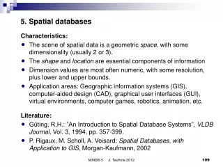
5. Spatial databases Characteristics: • The scene of spatial data is a geometric space, with somedimensionality (usually 2 or 3). • The shape and location are essential components of information • Dimension values are most often numeric, with some resolution, plus lower and upper bounds. • Application areas: Geographic information systems (GIS),computer-aided design (CAD), graphical user interfaces (GUI),virtual environments, computer games, robotics, animation, etc. Literature: • Güting, R.H.: ”An Introduction to Spatial Database Systems”, VLDB Journal, Vol. 3, 1994, pp. 357-399. • P. Rigaux, M. Scholl, A. Voisard: Spatial Databases, with Application to GIS, Morgan-Kaufmann, 2002 MMDB-5 J. Teuhola 2012
Abstract space modeling: Entity-based models Components of spatial objects: • identity • description • spatial extent Classification based on dimensionality: • Choice depends on the application viewpoint. (a) Zero-dimensional objects = points • Object does not have a shape, or it is not considered useful • Area quite small with respect to the embedding space,e.g. cities, buildings, road crossings on a map. • Depends e.g. on the scale of the map. MMDB-5 J. Teuhola 2012
Entity-based models (cont.) (b) One-dimensional = line objects • E.g. roads on a map • Main geometric type: polyline, consistingof a finite set of line segments (edges),so that each segment endpoint (vertex)is shared by exactly two segments,except the two endpoints (if any). • Simple polyline: no intersections. • Closed polyline: endpoints meet. • Any curve can be approximated arbitrarilyclosely with a polyline. MMDB-5 J. Teuhola 2012
Entity-based models (cont.) (c) Two-dimensional = surfacic objects • Represent entities with a non-zero area. • Main geometric type:Polygon = region bounded by a closed polyline. • Convex polygon:For any points A, B P, line segment AB is fully included in P. (d) Three-dimensional = volumetric objects (polyhedrons) (e) Four-dimensional = spatio-temporal objects MMDB-5 J. Teuhola 2012
Abstract space modeling:Field-based models • Called also space-based models • The spatial information is considered a continuous (though approximated) field, i.e. a function of coordinates (e.g. x and y). • Each point of space is associated with one or more attributes. • Examples: • temperature, air pressure, height from sea level etc. at different points on maps, see e.g.http://ilmatieteenlaitos.fi/ • grey-level in a grey-scale digital image • red, green and blue components in a true-color (photographic) digital image MMDB-5 J. Teuhola 2012
Representation modes of spatial objects Tessellation mode • Cellular decomposition (grid, mesh, tiling, etc.) • Fixed tessellation: regular grid (rastering) • Variable tessellation: different sizes of decomposition units • Regular/irregular tessellation • Default: N x M rectangular (usually square) cells, called pixels • Natural (discrete) representation for field-based data • Entity-based data: one pixel for points, a set of pixels for polylines and polygons. • A more precise representation requires more storage space, and its processing takes more time. MMDB-5 J. Teuhola 2012
Representation modes of spatial objects (cont.) Vector mode Natural for the entity model. • Representation primitives: points and edges • Polygon and polyline are both represented as lists of points • 2n representations for a polygon with n vertices (selection of starting vertex, clockwise/counterclockwise order) • A region is a set of polygons • Representation may be complemented by restrictions(e.g. to simple polygons) • Representing field-based data in vector mode;Digital Elevation Models (DEM): • Field values only for a subset of points • The rest of the values are interpolated. • Example: Triangulated Irregular Networks (TIN) MMDB-5 J. Teuhola 2012
Representation modes of spatial objects (cont.) Half-plane representation • Only a single primitive: half-plane (half-space generally) • Sound mathematical basis • Half-space definition in d-dimensional space: inequality a1x1 + a2x2 + ... + adxd + ad+1 0 • Convexpolygon = intersection of a finite number of half-planes. • Polygon = union of a finite number of convex polygons. • Line segment = convex polygon of dimension 1(intersection of two half lines or rays) • Polyline = union of some line segments MMDB-5 J. Teuhola 2012
Compatibility of models and representations Space model Entity-based Field-based Tessellation Represen- tation Vectors Half-planes Possible Natural Natural Possible Possible Unlikely MMDB-5 J. Teuhola 2012
Computational geometry: typical problems • Is a point inside a polygon? • Intersection of line segments • Intersections of polylines • Intersection of polygons • Windowing and clipping with a rectangle • Polygon triangulation • Polygon trapezoidalization • Partitioning of a polygon into convex sub-polygons MMDB-5 J. Teuhola 2012
Computational geometry:algorithmic techniques for big problems (a) Incremental algorithms • Solve the problem for a small subset of input and add the rest one by one, maintaining the solution at each step. (b) Divide-and-conquer strategy • Divide step: recursively split the task into subproblems, until those can be solved easily. • Conquer step: Merge the subproblem solutions bottom-up into a global solution. (c) Sweep-line method • Decompose the input into vertical strips, so that the information related to the problem is located on lines separating the strips. MMDB-5 J. Teuhola 2012
Storage and retrieval of spatial objects Preliminary issues: • Arbitrary shapes difficult to handle Restriction to axis-oriented Minimum Bounding Rectangles (MBR), called also Bounding Boxes (BB). • Dimensions are often transformed to the real interval [0, 1);the whole space is a hypercube, denoted Ek. Performance factors: • Selected data structure • Dimensionality of the space • Distribution of objects in space: • density at point P = number of rectangles containing P • global density = maximum of local densities. MMDB-5 J. Teuhola 2012
Illustration of MBRs MMDB-5 J. Teuhola 2012
Query types for spatial objects (1) Exact-match query: Not very common for spatial objects,except in the context of insert. (2) Point query: For a point P Ek, find all rectangles R in thedatabase such that P R. (3) Rectangle intersection: For a given rectangle S Ek, find allrectangles R with S R . (4) Rectangle enclosure: For a given rectangle S Ek, find allrectangles R with S R. (5) Rectangle containment: For a given rectangle S Ek, find allrectangles R with R S. (6) Volume query: Given v1,v2 (0,1) and v1v2, find allrectangles with volume within [v1,v2]. (7) Spatial join: For two sets of k-dimensional rectangles, find allrelated pairs, satisfying a given join condition, such asintersection, enclosure, or containment. MMDB-5 J. Teuhola 2012
Illustration of spatial join • Intersection-join of { R1, R2, R3 } and { S1, S2, S3, S4 } is{ (R1, S2), (R2, S2), (R3, S3) } S4 S2 R1 S1 R2 R3 S3 MMDB-5 J. Teuhola 2012
Transformation approach for organizing sets of spatial objects • k-dim. rectangle can be represented as a 2k-dimensional point. • Alternatives e.g. in 2-dim. space: (a) (cx, cy, ex, ey), where (cx, cy) is the center point and ex and eyare the distances of the center from the sides. (b) (lx, ly, ux, uy), where (lx, ly) is the lower left, and (ux, uy) is the upper right corner of the rectangle. • Advantage of alternative (a): Location coordinates cxand cy are distinct from extension coordinates ex and ey. Special case: • 1-dimensional space [0, 1) • Rectangle = Line segment [0, 1) • Alternative 2-dimensional representations: (a) (c, e) = (center, half of length) (b) (l, u) = (lower endpoint, upper endpoint) MMDB-5 J. Teuhola 2012
S3 e L4 S1 L3 u S4 0.5 L2 P1 S2 L1 P3 1 P2 P4 0 1 0 1 0 1 c l Example of the transformation approach Notes: • When PAMs are applied to transformed representation, they suffer from the empty triangles (so called dead regions). • The (center, extension) approach can be improved, if we know an upper bound to the rectangle side; the ‘live space’ will look like a trapezoid, and the dead triangles are relatively small. MMDB-5 J. Teuhola 2012
0.5 R S e R S R S R S R S = R S = 1 c Answering queries in the transformation approach • Successful areas for different types of queries can be derived by simple geometric calculations. • Example: 1-dim. rectangles (= line segments) represented as 2-dim. points using the (center, extension) approach; query rectangle S = (c, e): • Drawback: Close, but different-volume rectangles may be located quite far in 2k-dimensional space. MMDB-5 J. Teuhola 2012
R1 R41 R42 R31 R32 R51 R52 R33 R34 R2 R6 Clipping approach for organizing sets of spatial objects • Assumption: Space is partitioned into disjoint rectangular regions (such as with most PAMs). • A new rectangle R may be located in two main positions: • R is inside one region: Simple to handle (as in PAM). • R intersects at least two regions. • In clipping, each intersection piece is inserted as a separate rectangle, but all pieces point to the same actual object (stored elsewhere). MMDB-5 J. Teuhola 2012
Clipping approach: viewpoints Advantages: • Clipping can be implemented almost directly with any PAM • Points and rectangles can be stored in the same file Disadvantages: • Increased space demand (multiple pointers to the same object) • Increased insert and delete costs • Overflow pages are needed, if the global density is high Query performance: • Exact match, point and enclosure queries need only one page access, if there are no overflows. • Intersection and containment queries may require all pieces of the clipped query rectangle to be inspected. The number of false drops may be high. MMDB-5 J. Teuhola 2012
Overlapping regions for organizing sets of spatial objects • Each rectangle presented only once in the database. • Rectangles are grouped into disk pages. • A group region is represented by its Minimum Bounding Rectangle. • Regions may overlap. • Example: R5 R4 R1 R6 R2 R3 R10 R8 R9 R7 MMDB-5 J. Teuhola 2012
Overlapping regions: viewpoints Possible drawbacks: • High overlap deteriorates performance. • Overlap of MBRs may be much higher than overlap of the base rectangles. • Exact-match query, insert and delete may require accessing more than one data page. • Intersection and containment queries may require accesses to the same pages, though the latter has usually a much smaller result size (every contained rectangle also intersects). Generalization: • Regions (MBRs of groups) may be grouped further into higher-level rectangles. • A tree structure is thus formed. MMDB-5 J. Teuhola 2012
Index utilizing overlapping regions: R-tree R-tree = Rectangle tree (Guttman 1984) • Balanced, dynamic external tree structure, where node = page. • Used e.g. by Oracle spatial extension. Node types: • A leaf contains (R, ptr) pairs where R is the MBR of the actual spatial object, and ptr points to its precise representation. • An internal node contains (R, ptr) pairs, where R is the MBR of the rectangles in a child, and ptr points to that child. MMDB-5 J. Teuhola 2012
R15 R16 R13 R14 R9 R10 R6 R7 R8 R4 R5 R1 R2 R3 R11 R12 Example R-tree R11 R2 R15 R1 R3 R16 R7 R13 R6 R12 R5 R8 R14 R9 R4 R10 MMDB-5 J. Teuhola 2012
Properties of the R-tree • Bounding rectangles on the path from root to leaf are nested. • Otherwise, there are no restrictions for overlaps;however they should be minimized. • For page capacity M (entries), a lower bound mM/2 is defined for the number of entries per page. • For N entries, height logmN1, and number of nodes N/(m 1) MMDB-5 J. Teuhola 2012
R-tree: Basic queries (a) Point query: Find objects that contain a given point.From the root node, search all subtrees (recursively) whereMBR contains the point. From the leaf level we get pointers to candidate objects which are finally checked. (b) Intersection query: Find objects intersecting with the query rectangle. Processing is similar as in (a), but now the condition is overlap, not containment. Other query types are generalized in the same way. Performance: • No guarantee, because multiple paths may have to be followed. • The amount of overlap in index regions (corresponding to internal nodes.) determines the performance. The insert operation plays the most important role in minimizing the overlap. The splitting of pages at overflow should minimize the overlap of the halves. MMDB-5 J. Teuhola 2012
Other spatial index structures R*-tree: Improved version of R-tree (Beckmann et al, 1990) • Defers splitting of pages by using forced reinsert of rectangles that are the most remote from the center of page MBR. • Applies a more sophisticated O(M log M)-time splitting heuristic. • Outperforms R-tree • Good also as a PAM (in low-dimensional spaces) • A popular ‘reference structure’ for other spatial data structures. X-tree (Berchtold et al, 1996) • Outperforms R*-tree in high-dimensional spaces. • Adapts to the number of dimensions. • General conjecture: When the dimensionality of the space grows, a sequential index becomes more and more advantageous. X-tree solves this by using variable-size nodes. MMDB-5 J. Teuhola 2012
Geographic databases: vocabulary Geographic object: • Two components: • Descriptive component with alphanumeric attributes,e.g. city: name, population • Spatial component (called also spatial object) describes the geometry (location, shape), e.g. city: polygon in 2-dim. space. Atomic/complex geographic objects: • Complex object consists of other atomic/complex objects. Theme: • Class (type) of geographic objects. • Corresponds to a relation; it has a schema and instances. • Example themes: Rivers, cities, countries, roads. MMDB-5 J. Teuhola 2012
Geospatial operations Theme projection to a subset of descriptive attributes: • Corresponds to relational projection. • Visual effect: part of the map attributes are dropped. Theme selection on the basis of descriptive attributes: • Corresponds to relational selection. • Keeps only the geographic objects satisfying a selection condition. • Visual effect: part of the objects are dropped. Geometric selection: • Windowing selects objects intersecting with a given rectangle. • Point query selects objects whose geometry contains a given point. • Clipping differs from windowing in that only intersections,not whole geometric objects, are taken to the result. MMDB-5 J. Teuhola 2012
Geospatial operations (cont.) Theme union: • Corresponds to relational union. • Combines two themes having the same schema. Theme overlay: • A common operation in GIS applications. • Spatial join: compute intersections. • New geographic objects are created from intersections, with • descriptive attributes of both components, • spatial component being the geometric intersection. Metric operations, e.g.: • Distance between Turku and Helsinki. Topological operations, e.g.: • List countries adjacent to Finland (Sweden, Norway, Russia, Estonia) • List cities reachable by train from Turku without stops (Salo, Loimaa). MMDB-5 J. Teuhola 2012
Geospatial software products ArcGIS: • Group of tools for geographic information systems • Geodatabase is a central component - an object-relational implementation of spatial data. For internet applications: • ArcIMS (Esri) • Mapserver (open-source) • GeoServer (open-source) MMDB-5 J. Teuhola 2012
Geospatial extensions ro relational database systems Oracle Spatial: • SQL extended with operators on the spatial data type. • Spatial indexing • R-tree • Quadtree based on z-order numbering • Query optimization, e.g. for spatial joins. PostgreSQL: • ’Object-relational’ DBMS; open-source, popular • Extended features: • Geometric types: point, line, line segment, rectangle, open and closed polyline, polygon, circle. • Operations on geometric types: translation, scaling, various tests • Supports a generalized GiST index, with R-tree as special case • Further extension package: PostGIS MMDB-5 J. Teuhola 2012