Download
1 / 35
350 likes | 373 Vues
Learn about the importance of longitudinal dynamics in storage rings, beam transport in linacs, and applications like Free Electron Lasers. Explore the synchrotron motion in storage rings and RF synchronization concepts.

E N D
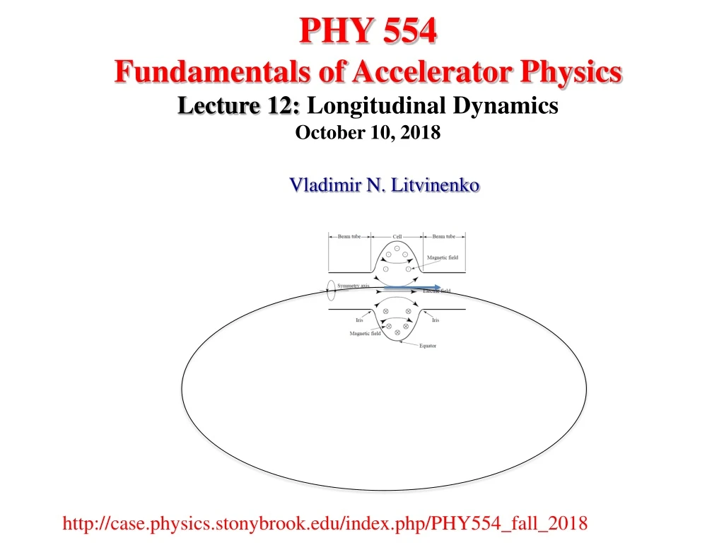
PHY 554 Fundamentals of Accelerator PhysicsLecture 12: LongitudinalDynamicsOctober 10, 2018 Vladimir N. Litvinenko http://case.physics.stonybrook.edu/index.php/PHY554_fall_2018
6-D Phase Space Acompletedescriptionofachargedparticlemotionwithrespecttothe‘idealparticle’mustbedonein 6D phase space. • Longitudinal dynamics is important in • Storage rings • Beam transport in linacs • Applications, such as Free Electron Lasers
Charged Particle passing an RF Cavity From previous lectures: Let us consider a ultra-relativistic particle passing a RF cavity, with the field E and voltage V. The energy gain of one charged particle with position z in a bunch: T(transit time factor)V
Synchrotron Motion in a Storage Ring • Longitudinal motion in circular accelerators is called synchrotron motion • The origin of this term originates from “synchrotron” where particles are “synchronized” with oscillating electric field in RF cavity(ies) • Similar to “betatron” motion name for transverse degrees of freedom, it is purely historical slang • Hence, the terminology is extended to synchrotron oscillations and synchrotron tune, Qs, for stable oscillations • In contrast with transverse motion, where particles typically execute multiple oscillations per tur, synchrotron oscillations are usually very slow with Qs <<1 • The later is used for a simplified description of slow synchrotron oscillations by separating them from “fast” betatron oscillations
RFSynchronizationinaring Thefrequencyofthe cavitymustbe integer harmonic of the revolution frequency: Circumference:C Revolutionfrequency:ω0 hiscalledharmonicnumber. hidealparticles cancirculateinthering. They are called synchronous particles
Charged Particle in RFCavityII • We name the synchronous particle’s phase • For a number of good reasons we don’t want the particle to experience the highest accelerating voltage (on crest).
Energy change by the RF cavity Synchronous particle energy change in the cavity is given by its synchronous phase Non-zero value of energy change can be related to acceleration/deceleration of the beam or compensation for energy losses in the ring (such as radiation losses) The energy of a particle displaced by distance z from synchronous particle changes as Using relative values, we can re-write the above equations in dimensionless form δ changes between nth to (n+1)th turn in the ring as: Now we know, how the energy deviation evolves
Revolution time of a particle • Let’s consider the consequence of the energy deviation • Its velocity changes: • And the pass length change • The arrival time difference ds(1+ Dδ/ρ) ρ ds ρ+Dδ
Change in RF phase Then we can translate the arriving time to the rf phase variable: Change to turn by turn mapping format: Combined with the earlier change in the energy change, we have the longitudinal one-turn map:
Fixed Points • For any nonlinear map the first step is attempt to find fixed point(s) • The fixed point is defined as: • And located at • Next step to find iffixed points are stable are not?
An Example • Consider the example with following parameter: • Proton beam with 100 GeV or 15 GeV • Cavity voltage 5 MV,360harmonic • Compaction factor 0.002 • Nonetacceleration. • Initial condition:
From Map to Hamiltonian Finite differential map: Can be approximately described by differential equations when variations are small with the turn number as independent variable and an effective Hamiltonian of a pendulum!
Similarity to pendulum@ zero accelerating phase ‘MASS’ (not unique) Stable phase Bucket height For stable motion Angular frequency for small oscillation
Small amplitude approximationStability criterion Back to the 2nd order differential equation For small phase deviations we can linearize it And find stability condition:
Synchrotron tune The ‘tune’ is extracted as • Typical Numbers • Hadron rings: Qs ~ 10-3 • Electron rings: Qs ~ 10-2 Synchrotron tune for zero crossing
Small Amplitude ApproximationHamiltonian When the phase is close enough to the synchronous phase: The phase space trajectory will be upright ellipse for fixed ‘energy’
Transition energy Transition happens when: Below transition: Faster particle arrives first Above transition: Slower particle arrives first
Physics Picture Above Transition Below Transition
Non-zero acceleration phase • In lepton (electron & positron) storage rings, as well in future high (TeVs) energy hadron rings , we need acceleration for synchronous particle to compensate energy loss. • For now, we assume that the energy loss per turn is energy independent, and not net acceleration for synchronous particle. Stable region Effective potential
Phase space 15 GeV 100 GeV
Longitudinal Phase Space • We can define longitudinal phase space area from the conjugate variables. • The phase space area remain constant even in acceleration • If we stay with, , the phase space area is constant only without net acceleration.
Longitudinal Phase Space II • We may take a Gaussian beam distribution then the rms phase space area is simply: • The area is conserved only • When the beam distribution matches the bucket • When the beam oscillation is very small (linear).
Phase Space AreaExamples and Evolution I A Matched case (Perfect injection): Initial conditions match:
Phase Space AreaExamples and Evolution II An unmatched case
Phase Space AreaExamples and Evolution III Time jitter at injection, other wise same as the matched case: The phase error is:
What we learned today? • Stable longitudinal (e.g. energy – arrival time) motion of particles in circular accelerators is called synchrotron oscillations • Synchrotron motion is described with respect to a synchronous (ideal, or moving as designed) particle, which may experience acceleration, deceleration or energy loss by various processes such as radiation • RF frequency is a integer harmonic (h) of the synchronous particle revolution frequency and has to be adjusted if velocity of the beam changes • h bunches can be operated (accelerated) simultaneously in such storage ring/synchrotron. Area in energy-phase space for each bunch is called “RF bucket” • There two phases for synchronous particles in each RF bucket: one stable and one unstable (saddle) • Stable phase (positive or negative slope) depends on sign of the slip factor η. The slip factor depends on the particles energy: the energy where η crosses zero is called critical energy. Typically transition energy occurs when relativistic factor γ~Qx • Crossing critical energy in accelerators is challenging and requires a number of sudden lattice modification to keep beam stable. Lepton ring are typically operate above the transition energy and do not have such complications • has time independent Hamiltonian (e.g. it is a constant!) and use the Hamiltonian contour plot as
What we learned today? • Accurate description of synchrotron motion is described by a map, e.g. change of the energy and the phase in finite differentials. Synchrotron oscillation have stability areas separated by trajectory (called separatrix) from area of unstable motion. • Synchrotron oscillations are typically very slow, Qs<<1, which allows to describe them by differential equation identical that that of a pendulum. Such description has time independent Hamiltonian (e.g. it is a constant!) and use the Hamiltonian contour plot as particles trajectories in the phase space • When synchronous particles have zero energy change in RF cavity (no acceleration, no energy loss), separatrices a symmetric and particles outsize the separatrix acceptance are drifting in phase without being “lost”: particles with higher energy above the separatrix never cross to the lower part and vice versa. E-Eo t
What we learned today? E-Eo • When synchronous particles gaining or losing energy, topology of the phase space changes: particles can cross from the upper part to the bottom part (typical for qn acceleration or a energy loss case) or from the bottom to top (for a deceleration case) – these particles will be lost by hitting energy acceptance of the lattice • Synchrotron oscillations are intrinsically nonlinear and asynchronous: oscillations with larger amplitudes are slower than at small amplitudes. Period turns into infinity at the separatrix: particle never reaches a saddle point. • Pair (-t, E) is a canonical pair and Liouville theorem guaranties preservation of the phase space occupied by particles • During injection of particles, phase and energy errors as well as mismatch of the particles distribution can lead to effective “emittance” growth by particles entrapping “empty space”. Asynchronousity of oscillations is the cause of this mixing. t
Credits • This lecture is an updated version of 2016 lecture on the same subject prepared by Prof. Yue Hao (now at MSU) • The most important credit to Prof. Yue Hao are for the animations of the particles motions in slides 29-31


