Download

1 / 37
370 likes | 537 Vues
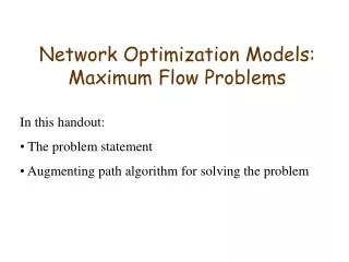
Maximum Network Flow by me Dr. M. Sakalli Ch26 of CSLR and many other sources. Marmara Univ. Chapter 26 of CLSR. a. 2/15. 4/19. t. s. 2/5. 0/9. 3/3. 5/14. b. A Flow Network, terminology. Modeled as a flow graph which is a directed graph of G= ( V,E ) .

E N D
Maximum Network Flowby me Dr. M. Sakalli Ch26 of CSLR and many other sources. Marmara Univ. Chapter 26 of CLSR
a 2/15 4/19 t s 2/5 0/9 3/3 5/14 b A Flow Network, terminology • Modeled as a flow graph which is a directed graph of G=(V,E). • Flow– a function f : V ´V ® R: Rate passing through the network from the source vertex s to the sinking vertex t. In literature called as s-t network. Net flow, |f(u,v)|. • Source is vertex from which all the edges are leaving ‘s’, and sink is the vertex, all the edges incident to ‘t’.
A Flow Network, Constraints A flow is an assignment of real numbers xij to edges (i,j) of a given network that satisfy the following: flow-conservation requirements and capacity constraints Capacity constraint: Each edge has a maximum capacity ‘ce’ allowed to transmit through such that.. Net flow cannot exceed ce… u, v ÎV: f(u, v) £ c(u, v) Skew symmetry constraint: u, v ÎV:f(u,v) = –f(v,u) Flow conservation Law: The sum of the net flow incident to a vertex is equal to the net flow leaving the same vertex. u, v ÎV – {s, t}, ΣvVf(u, v)=0. for entire vertices. What goes in = what leaves out: ΣvVf(u, V)- ΣvVf(V, v) =0, s and t vertices: ΣvVf(v, s)=0, ΣvVf(t, v)=0, ΣvVf(s, v) = ΣvVf(v, t)>0 and R+, No leakage and no memory is allowed. Total value of flow, |f| = f(s, V) = f(V, t) Among the areas applied are traffic, freight, airflow, hydrodynamic, communications, and stocks, companies. The Maximum Flow Problem Definition: is to find a feasible flow through a single-source, single-sink flow network that is maximum. a 2/15 4/19 t s 2/5 0/9 3/3 5/14 b
2/13 a b 2/19 3/15 1/10 t 1/4 9 1/5 s 1/14 3/11 2/3 c d • Opposite flows bt two vertices (due to skew symmetry) will cancel each other. • Super source and super sink connected with infinite capacity. • Find paths to maximize |f|. • f(X, Y) means ΣxXΣyYf(x, y) • f(u, V – {s, t}) = 0 Max Flow, |f| = 19 Or is it? Best we can do? Lucky Puck Distribution Network
a a 2/15 5/19 2/15 5/19 t t s s 0/9 5/5 2/9 3/5 2/3 2/3 5/14 5/14 b b • For X, Y, Z V with X Y =, • f(XY, Z) = f(X, Z) + f(Y, Z) flow between any x and y through Z…. • f(Z, X Y) = f(Z, X) + f(Z, Y) • The value of a flow is the total net flow into the sink; that is, |f|= f(V, t), and from the source s |f| = f(s, V) (by definition) = f(V-{V-s}, V) = f(V, V) - f(V - s, V) = f(V, V - s) |f|= f(V, t) = f(V, t) + f(V, V - s - t) = f(V, t) (by flow conservation) Cancellation of flows
Ford-Fulkerson method • Initialize flow value to 0. Start to iterate (dynamic or greedy!).. • Find augmenting paths • Find a path p from s to t, such that there is some flow value x > 0, and for each edge (u, v) in p, add x units of flow to |f|, such that max{x} min{cf(u, v): (u, v) is on p}. • Increment flow, f(u, v) = f(u, v) + x • Calculate residual capacities: cf(u,v) = c(u,v) – x i.e. the actual capacity minus the net flow (x) from u to v Flow may be negative!! That can be interpreted as increasing residual capacity. • Residual network: Gf =(V, Ef), where Ef = {(u,v) ÎV ´ V : cf(u,v) > 0} • Continue till no any augmenting path (any forward channel) left through • Observation – edges in Ef are either edges in E or their reversals: |Ef| £2|E| Augmenting Path? 13 19 a b 15 10 t 5 9 s 4 14 11 3 d c
Ford-Fulkerson method Contains several algorithms: Residue networks Augmenting paths Find a path p from s to t (augmenting path), such that there is some value x > 0, and for each edge (u,v) in p we can add x units of flow f(u,v) + x c(u,v) Augmenting Path? 8/13 a b 10/15 13/19 10 t s 5/5 9 2/4 6/14 8/11 3/3 c d
Residual Network To find augmenting path we can find any path in the residual network: Residual capacities: cf(u,v) = c(u,v) – f(u,v) i.e. the actual capacity minus the net flow from u to v Net flow may be negative Residual network: Gf =(V,Ef), where Ef = {(u,v) ÎV ´V : cf(u,v) > 0} Observation – edges in Ef are either edges in E or their reversals: |Ef| £2|E| 5/15 10 Residual Sub-Graph Sub-graph With c(u,v) and f(u,v) a b 5/6 a b 1 c c 0/14 19 5
Residual Graph Compute the residual graph of the graph with the following flow: 8/13 a b 10/15 13/19 10 t s 5/5 9 2/4 6/14 8/11 3/3 c d
Residual Capacity and Augmenting Path Finding an Augmenting Path Find a path from s to t in the residual graph The residual capacity of a path p in Gf: cf(p) = min{cf(u,v): (u,v) is in p} i.e. find the minimum capacity along p Doing augmentation: for all (u,v) in p, we just add this cf(p) to f(u,v) (and subtract it from f(v,u)) Resulting flow is a valid flow with a larger value.
Residual network and augmenting path f(p1:(s, v1),…) = 11, as far as cf(s,v1)<16, and as far as sum v1=0, and f(p2:(s, v2),…), calculate final residual graph Gf, and next search augmentation path.
The Ford-Fulkerson method Ford-Fulkerson(G,s,t) 1 for each edge (u,v) in G.E do 2 f(u,v) ¬ f(v,u) ¬ 0 3 while there exists a path p from s to t in residual network Gfdo 4 cf = min{cf(u,v): (u,v) is in p} 5 for each edge (u,v) in p do 6 f(u,v) ¬ f(u,v) + cf 7 f(v,u)¬-f(u,v) 8 return f The algorithms based on this method differ in how they choose p in step 3. Steps 1, 2, O(E), and 4-7 O(E) times for each unit of |f*|. If chosen poorly the algorithm might not terminate.
Execution of Ford-Fulkerson (1) Left Side = Residual Graph Right Side = Augmented Flow
Execution of Ford-Fulkerson (2) Left Side = Residual Graph Right Side = Augmented Flow
Path augmenting scenarios Fig 27.4 of CLSR: The flow network G with f. The residual network Gf with augmenting path p shaded; its residual capacity is cf(p) = c(v2, v3) = 4. (c) The flow in G that results from augmenting along path p by its residual capacity 4. (d) The residual network induced by the flow in (c).
The Ford-Fulkerson algorithm, Residual Capacity and Augmenting Path In each iteration find any path augmenting the flow along by the residual capacity câ(p). Following algo computes the max f in G = (V, E) by updating the net â[u, v] between connected vertices; u, v. If not connected, implicit assumption is that â[u, v] = 0. Assumption: the c(u, v) is a constant-time function, which is 0 if (u, v) E. c(u, v) might be derived from fields stored within vertices and their adjacency lists. The residual capacity: câ(u, v).. Here the câ(p) is a temporary variable for the câ(u, v) of the path p. () refers a function [] refers a mutable identifier. Ford-Fulkerson(G,s,t) 1 for each edge (u,v) G.E do //Initializing 2 f(u,v) ¬ f(v,u) ¬ 0 3 while path p from s to t in residual network Gf do *** 4 cf = min{cf(u,v): (u,v) p}// determining augmentation 5 for each edge (u,v) p do// updating residual capacities, new Gf 6 f(u,v) ¬ f(u,v) + cf 7 f(v,u)¬-f(u,v) 8 return f T(n) depends on how line 3 is implemented and the algorithms based on this differ in how to determine p. If chosen poorly the algorithm might not terminate. http://www-b2.is.tokushima-u.ac.jp/~ikeda/suuri/maxflow/Maxflow.shtml
Residual Graphs Augmented Flow Execution 12 20 a b 16 9 t 7 10 s 4 13 14 4 d c
Residual Graph Augmented Flow Execution of Ford-Fulkerson 12 a b 1/19 5/11 9 t 7 3/11 s 13 4 3/11 d c Observe that terminates when there is no a path from s to t whose all edges are in forward direction. And observe that the edges whose capacities are depleted form bottleneck, which is the minimum cut and their total capacity of the maximum achivible.
Does the method find the maximum flow? Yes, if program can get to the point where the residual graph has no path from s to t. Which is the moment when the G(V, E) is partitioned into two disjoint sets, by a definite split, minimum cut, c(S, V-S) = c(S, T), such that s S and t T. • And the net flow (f(S,T)) through the cut (or the capacity) is the total capacity of the flows f(u,v), where s S and t T which includes negative flows back from T to S as well.Think about it from the graph… • Minimum cut – a cut with the smallest capacity of all cuts. |f|= f(S,T) i.e. the value of a max flow is equal to the capacity of a min cut. 8/13 a b 10/15 13/19 10 t s 5/5 9 2/4 6/14 8/11 3/3 c d Cut capacity = 24 Min Cut capacity = 21
Cut properties.. • A cut (S, T) of flow network G = (V, E) is a partition (or a disjoint set) of V into S and T = V - S such that s S and t T. MST cut was for undirected graphs, here a directed graph is cut such that (tails) s S and (heads) t T.) If f is a flow, then the net flow across the cut (S, T) is defined to be â(S, T). The capacity of the cut (S, T) is c(S, T). • f(S, T) = ΣuSΣvTf(u, v) ΣuSΣvTc(u, v) = c(S, T). • The value of any flow â in a flow network G is bounded from above by the capacity of any cut of G. • Proof Let (S, T) be any cut of G and let â be any flow. By |â| = â(S, T) (Lemma 27.5 clrs) and the capacity constraints, • = ΣuSΣvTf(u, v)ΣuSΣvTc(u, v) = c(S, T)
Max-flow min-cut theorem If f is a flow in a flow network G=(V, E) with source s and sink t, then the following conditions are equivalent: 1. f is a maximum flow in G. 2. The residual network Gf contains no augmenting paths. 3. Flow value of f = c(S, T) for some cut (S,T) of G. (This cut is called min-cut. Bottleneck. Among all the cuts of G(S, T), it is the cut that returns the minimum capacity.)
Proof 1→2 Use contradiction. If it does not hold, then the residual network Gf must have some augmenting paths. So the net flow |f| could be further increased which contradicts to that |f| is a maximum flow in G. 2→3 Suppose that Gf has no augmenting path, that is, that Gf contains no path from s to t. Define S={vV: there exists a path from s to v in Gf} and T=V-S. The partition (S,T) is a cut: we have s S trivially and tT because there is no path from s to t in Gf. For each pair of vertices u and v such that uS and vT, we have f(u,v)=c(u,v) since otherwise (u,v)Ef, which would place v in set S. Thus, flow value of f=c(S,T). (Lemma: flow value f=f(S,T))
The end of Proof 3→1 The value of any flow f in a flow network G is bounded from above by the capacity of any cut of G. flow value f(S, T)=ΣuSΣvTf(u, v) ΣuSΣvTc(u, v) = c(S, T). so the cut capacity c(S,T) is the upper bound of flow f. Now the flow value f=c(S,T) thus implies that f is a maximum flow.
v 1000000 1000000 p1 s 1/1 t 1000000 1000000 u v 1/1000000-1 1000000 p2 1 s t 1000000-1/1 1000000 u 1000000-1/1 v 1000000-1/1 p1 s 1 t 1/1000000-1 1/1000000-1 u Worst case analysis • In the worst case, suppose that at each step Ford-Fulkerson’s algorithm performs some small incremental (integer) augmentations of ∆f, then the number of iterations to reach to the maximum flow, |f*|/∆f, where f* is maximum flow. • In the given example (clrs) programs starts to traverse through path p1, suvt and alternates to the path p2, svut. instead of completing the algorithm in two steps. • The running time of Ford-Fulkerson’s algorithm is O(|f*|(E))
Edmonds-Karp algorithm • If searching path p in line 3, is implemented with a BFS in the residual network, and if the augmentation path is a shortest path from s to t, regardless of the weights of edges, • Edmonds-Karp algorithm. O(VE2), take shortest augmentation path. • How do we find such a shortest path? DFS or BFS.. • The number of augmenting paths needed by the shortest-augmenting-path algorithm never exceeds nm/2, where n and m are the number of vertices and edges, respectively • Since the time required to find shortest augmenting path by breadth-first search is in O(n+m)=O(m) for networks represented by their adjacency lists, the time efficiency of the shortest-augmenting-path algorithm is in O(VE2) or O(nm2) for this representation. • Running time O(VE2), because the number of augmentations is O(VE) • More efficient algorithms have been found that can run in close to O(nm) time • BFS and AP and Maximum Capacity Path (MCP) - find an A.P. that maximizes incremental flow • How many augmenting paths for each method? • Edmonds-Karp - A.P.s to give overall time. • Critical edge on A.P. No capacity will remain on a critical edge after A.P. is recorded • Observations: Edge may become critical several times. A vertex cannot get closer to source in later rounds of BFS.
First time critical Later • Each augmentation has complexity O(E) • Numbers of augmentations is O(VE) • Each edge can be a critical edge at most |V|/2-1 times • Once edge is critical, its flow is saturated • Must appear in path the other way next • Since previous path is shortest, this reversing path must be two edges longer df’(s,v)=df(s,u)+1 df’(s,u)=df’(s,v)+1 ≥df(s,v)+1 (paths increase monotonically) =df(s,u)+2 Second time critical The number of distances available for the tail of a repeated critical edge is (V-2)/2. The number of edges that become critical is <E. Thus, A.P.s overall. Flow must be sent in opposite direction by another A.P. before an edge can become critical again.
Shortest-Augmenting-Path Algorithm Generate augmenting path with the least number of edges by BFS. Start at s, perform BFS traversal by marking new (unlabeled) vertices with two labels and a sign mark: • 1st label – indicates the amount of additional flow that can be brought from the previous to the current vertex being labeled. • 2nd label – indicates the vertex from which the vertex being labeled was reached, with “+” or “–” in forward or in backward, respectively. • Vertex labeling:The start is always labeled with ∞,- • All other vertices are labeled as follows: If unlabeled vertex j is connected to the front vertex i with the edge • from i to j with unused capacity rij = uij –f(uij, vij) (forward edge), vertex j is labeled with lj, i+, where lj = min{li, rij}. • from j to i with positive flow xji (backward edge), vertex j is labeled lj,i-, where lj = min{li, xji}
2,2+ 5 5 0/3 0/4 0/3 0/4 2,1+ ∞,- 0/2 0/5 0/2 s 2 3 t 0/2 0/5 0/2 s 2 3 t 2,2+ 2,3+ 0/3 0/1 0/3 0/1 4 3,1+ 4 • If the sink ends up being labeled, then there is an augmentation path by the amount min{cp} which indicated is with the sink’s first label. • The augmentation path is traced along the path from sink to source; the current flow quantities are increased on the forward edges and decreased on the backward edges of this path. • If the sink remains unlabeled after the traversal queue becomes empty, the algorithm returns the current flow as maximum and terminates. Queue: 1 2 4 3 5 6 ↑↑ ↑ ↑ Augment the flow by 2 (the sink’s first label) along the path 1→2→3→6
5 0/3 0/4 2/2 2/5 2/2 s 2 3 t 0/3 0/1 1,2+ 4 5 0/3 0/4 ∞,- 1,3- 1,4+ 2/2 2/5 2/2 s 2 3 t 1,5+ 0/3 0/1 4 3,1+4 Queue: 1 4 3 2 5 6 ↑↑ ↑ ↑ ↑ 5 1/3 1/4 Augment the flow by 1 (the sink’s first label) along the path 1→4→3←2→5→6 2/2 1/5 2/2 s 2 3 t 5 1/3 1/1 1/3 1/4 4 ∞,- 2/2 1/5 2/2 s 2 3 Queue: 1 4 ↑↑ t 1/3 1/1 4 2,1+ No augmenting path (the sink is unlabeled) the current flow is maximum
S : (∞, 1, +) • B : (S, 8, +) • E : (S, 28, +) • F : (S, 15, +) • A : (B, 8, +) • C : (B, 8, +) • D : (B, 6, -) • T : (A, 8, +) • f updated by 8. P = (S,B, A, T)
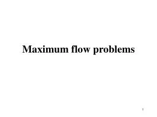
Multiple Sources or Sinks • What if you have a problem with more than one source and more than one sink? • Modify the graph to create a single supersource and supersink 13 a 13 b 15 13 a b 15 13 10 k 10 i 5 t 9 4 s 5 9 4 14 11 3 14 11 3 c d c d t s 4 4 13 e 13 f 15 13 e f 15 13 10 l 10 j 5 y 9 4 x 5 9 4 14 11 3 14 11 3 g h g h
Application – Bipartite Matching • Example – given a community with n men and m women • Assume we have a way to determine which couples (man/woman) are compatible for marriage • E.g. (Joe, Susan) or (Fred, Susan) but not (Frank, Susan) • Problem: Maximize the number of marriages • No polygamy allowed • solve this problem by creating a flow network out of a bipartite graph
Bipartite Graph • A bipartite graph is an undirected graph G=(V,E) in which V can be partitioned into two sets V1 and V2 such that (u,v) E implies either u V1 and v V2 or vice versa. • That is, all edges go between the two sets V1 and V2 and not within V1 and V2.
Model for Matching Problem • Men on leftmost set, women on rightmost set, edges if they are compatible A A A X X X B B B Y Y Y C C C Z Z Z D D D Men Women Optimal matching A matching
Solution Using Max Flow • Add a supersouce, supersink, make each undirected edge directed with a flow of 1 A A X X B B t Y s Y C C Z Z D D Since the input is 1, flow conservation prevents multiple matchings