Lumped Parameter Modelling
Lumped Parameter Modelling. P. Lewis & P. Saich RSU, Dept. Geography, University College London, 26 Bedford Way, London WC1H 0AP, UK. Introduction. introduce ‘simple’ lumped parameter models Build on RT modelling RT: formulate for biophysical parameters LAI, leaf number density, size etc

Lumped Parameter Modelling
E N D
Presentation Transcript
Lumped Parameter Modelling P. Lewis & P. Saich RSU, Dept. Geography, University College London, 26 Bedford Way, London WC1H 0AP, UK.
Introduction • introduce ‘simple’ lumped parameter models • Build on RT modelling • RT: formulate for biophysical parameters • LAI, leaf number density, size etc • investigate eg sensitivity of a signal to canopy properties • e.g. effects of soil moisture on VV polarised backscatter or Landsat TM waveband reflectance • Inversion? Non-linear, many parameters
Linear Models • For some set of independent variables x = {x0, x1, x2, … , xn} have a model of a dependent variable y which can be expressed as a linear combination of the independent variables.
Linear Mixture Modelling • Spectral mixture modelling: • Proportionate mixture of (n) end-member spectra • First-order model: no interactions between components
Linear Mixture Modelling • r = {rl0, rl1, … rlm, 1.0} • Measured reflectance spectrum (m wavelengths) • nx(m+1) matrix:
Linear Mixture Modelling • n=(m+1) – square matrix • Eg n=2 (wavebands), m=2 (end-members)
r1 r2 Reflectance Band 2 r r3 Reflectance Band 1
Linear Mixture Modelling • as described, is not robust to error in measurement or end-member spectra; • Proportions must be constrained to lie in the interval (0,1) • - effectively a convex hull constraint; • m+1 end-member spectra can be considered; • needs prior definition of end-member spectra; cannot directly take into account any variation in component reflectances • e.g. due to topographic effects
Linear Mixture Modelling in the presence of Noise • Define residual vector • minimise the sum of the squares of the error e, i.e. Method of Least Squares (MLS)
Error Minimisation • Set (partial) derivatives to zero
Error Minimisation • Can write as: Solve for P by matrix inversion
x x1 x2 y x
Weight of Determination (1/w) • Calculate uncertainty at y(x)
Lumped Canopy Models • Motivation • Describe reflectance/scattering but don’t need biophysical parameters • Or don’t have enough information • Examples • Albedo • Angular normalisation – eg of VIs • Detecting change in the signal • Require generalised measure e.g cover • When can ‘calibrate’ model • Need sufficient ground measures (or model) and to know conditions
Model Types • Empirical models • E.g. polynomials • E.g. describe BRDF by polynomial • Need to ‘guess’ functional form • OK for interpolation • Semi-empirical models • Based on physical principles, with empirical linkages • ‘Right sort of’ functional form • Better behaviour in integration/extrapolation (?)
Linear Kernel-driven Modelling of Canopy Reflectance • Semi-empirical models to deal with BRDF effects • Originally due to Roujean et al (1992) • Also Wanner et al (1995) • Practical use in MODIS products • BRDF effects from wide FOV sensors • MODIS, AVHRR, VEGETATION, MERIS
Satellite, Day 1 Satellite, Day 2 X
Model parameters: Isotropic Volumetric Geometric-Optics Linear BRDF Model • Of form:
Model Kernels: Volumetric Geometric-Optics Linear BRDF Model • Of form:
Volumetric Scattering • Develop from RT theory • Spherical LAD • Lambertian soil • Leaf reflectance = transmittance • First order scattering • Multiple scattering assumed isotropic
Volumetric Scattering • If LAI small:
Similar approach for RossThick Volumetric Scattering • Write as: RossThin kernel
Geometric Optics • Consider shadowing/protrusion from spheroid on stick (Li-Strahler 1985)
Geometric Optics • Assume ground and crown brightness equal • Fix ‘shape’ parameters • Linearised model • LiSparse • LiDense
Retro reflection (‘hot spot’) Kernels Volumetric (RossThick) and Geometric (LiSparse) kernels for viewing angle of 45 degrees
Kernel Models • Consider proportionate (a) mixture of two scattering effects
And uncertainty via BRDF Normalisation • Fit observations to model • Output predicted reflectance at standardised angles • E.g. nadir reflectance, nadir illumination • Typically not stable • E.g. nadir reflectance, SZA at local mean
Linear BRDF Models for albedo • Directional-hemispherical reflectance • can be phrased as an integral of BRF for a given illumination angle over all illumination angles. • measure of total reflectance due to a directional illumination source (e.g. the Sun) • sometimes called ‘black sky albedo’. • Radiation absorbed by the surface is simply 1-
Linear BRDF Models for albedo • Similarly, the bi-hemispherical reflectance • measure of total reflectance over all angles due to an isotropic (diffuse) illumination source (e.g. the sky). • sometimes known as ‘white sky albedo’
Spectral Albedo • Total (direct + diffuse) reflectance • Weighted by proportion of diffuse illumination Pre-calculate integrals – rapid calculation of albedo
Linear BRDF Models to track change • E.g. Burn scar detection • Active fire detection (e.g. MODIS) • Thermal • Relies on ‘seeing’ active fire • Miss many • Look for evidence of burn (scar)
Linear BRDF Models to track change • Examine change due to burn (MODIS)
MODIS Channel 5 Observation DOY 275
MODIS Channel 5 Observation DOY 277
Detect Change • Need to model BRDF effects • Define measure of dis-association
MODIS Channel 5 Prediction DOY 277
MODIS Channel 5 Discrepency DOY 277
MODIS Channel 5 Observation DOY 275
MODIS Channel 5 Prediction DOY 277
MODIS Channel 5 Observation DOY 277
Detect Change • Burns are: • negative change in Channel 5 • Of ‘long’ (week’) duration • Other changes picked up • E.g. clouds, cloud shadow • Shorter duration • or positive change (in all channels) • or negative change in all channels